


 Inglês (pdf)
 Artigo em XML
 Referências do artigo
 Enviar este artigo por email
 Citado por SciELO
  Citado por Google
  Similares em
SciELO
Similares em
SciELO  Similares em Google
 Permalink
1. introduction
The problem of position control has been widely treated in control literature; in fact, it is a ubiquitous classical example in every control-related textbook. In particular the position/velocity control has been important in the development of applications nowadays common in the human lifestyle; it covers the simplest objects as reading heads of hard drives [1,2], robotic manipulators with many degrees of freedom, electro-hydraulic devices [3,4], etc.
This paper aims to design and implement a position tracking controller for a DC motor. The control system must guarantee the performance characteristics required. To this aim, two control laws are designed and implemented: a) a model based methodology, and main focus of the paper, called Embedded Model Control (EMC) and b) a classical methodology based on feedback of tracking error without model knowledge. Many control schemes feature disturbance rejection and uncertainty. Among others, it is possible to find the so called Active Disturbance Rejection Control (ADRC) [5, 6] or Disturbance-Observer-Based Control (DOBC) [2]. Both schemes consider the existence of extended observers, in some flavors called Extended State Observer (ESO) [7,8] where a non-linear analysis was included, in others described las an special PI observer, Generalized Proportional Integral (GPI) observers [9,10] the Perturbation Observer (POB) [11], etc. All them have in common that they are enriched with additional dynamics able to store and reproduce in some way the aspects not covered by the model. Same structure follows the EMC where further issues have been already covered [12]. In [13] a comparative study between some model based schemes is presented. The main difference between ADRC and EMC is that the former assumes that model errors can be treated like input disturbances whereas EMC shows that high-frequency neglected dynamics cannot be treated as such. The former standpoint does not place any limitation to the control bandwidth (BW) unlike the latter one which is compelled to find out an optimal BW in the presence of uncertainty. A further comparison between ODBC and ADRC was presented in [10] together with some theorems and description of the ADRC/ODBC. In general most of these approaches share the same idea; they present a structure of two degrees of freedom, where one is in charge of achieving disturbance estimation for real-time rejection and the other provides the closed-loop performance and stability characteristics.
One goal of the EMC is to offer a way of converting model and control architecture into real-time code taking for granted that model and control architecture should not be completely free but constrained and guided by some basic principles (axioms and propositions) such as for instance, that the sole feedback channel passes through the noise vector or the core of a control unit is the embedded model [14]. The EMC has been applied to solve control problems that are challenging due to their complexity, uncertainty and high levels of precision like drag free satellites formation control, complex hydraulic systems [3] and complex instrumentation with submicron precision. In this paper a case study on a commercial platform is presented. The authors consider that this will provide with a benchmark example to be implemented easily by industrial practitioners, industrially related academics and researchers; which allows a deeper understanding of the control methodology and limitations.
The paper is organized as follows: the section 0 presents the case study, a brief description and physical modelling of the system as well as the definition of requirements to the control system. Section 0 presents the main characteristics of the EMC showing at each stage the application of the EMC to the case study and presenting the analysis and development of each component of the controller. Section 0 shows a brief summary of the PID design. Finally section 0 presents a set of tests and experimental results.
2. The case study: Educational Servo Motor
This section presents the case study where all test reported are conducted. Control systems are designed for position trajectory tracking of a servo motor. The plant under study is a didactic servo motor manufactured by Quanser® [15]. The system is composed by a DC motor driven by a PWM signal and an incremental encoder for position measurement.
2.1. Design model
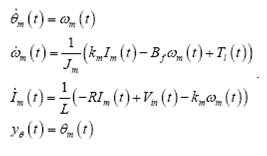
Angular displacement model is given by
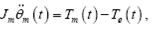 (1)
(1)
where Tm (t ) is the torque generated by the electrical element given by
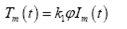 (2)
(2)
and Te (t ) the sum of viscous friction and load torque T (t ),
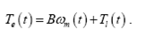 (3)
(3)
Derivatives of angular position θm (t ) are represented in terms of angular frequency ωm (t ) interchangeably. The armature circuit model is given by
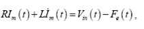 (4)
(4)
where, Im (t ) , Vn (t ) and ωm (t ) are the inductance current, voltage input and angular frequency respectively. The back EMF (electro motive force) is defined by
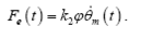 (5)
(5)
Under a constant flux and by assuming maximum efficiency  the model can be written as
 (6)
(6)
Angular position is limited to
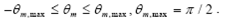 (7)
(7)
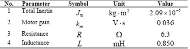
Process parameters are summarized in Table 1.
2.2. Control requirements
Control requirements are summarized next. Given a reference angular position signal yr (t ), the shaft angular position θm (t ) is delayed and modified as follows
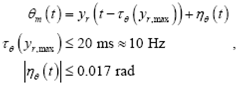 (8)
(8)
where
ηθ (t
) is the residual tracking error defined as the difference between the total tracking error 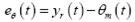 and the nominal tracking error
  imposed by the target delay
  and the performance rate
yr (t
), i.e.,
and the performance rate
yr (t
), i.e.,
 (9)
(9)
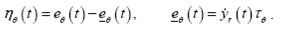
Continuous time notation is used since it is expected these requirements must be fulfilled by true angular position. However, errors are calculated and used by the controller from discrete time signals and measurements, as it will be shown in section 0. The disturbance rejection requirements are expressed in frequency terms, using the sensitivity function
 (10)
(10)
where ωrd correspond to the common called 0dB output disturbance rejection (Sensitivity) bandwidth.
3. The embedded model control
The EMC is a model based control methodology defined initially in [16] with notable improvements over the years [14]. Disturbance cancelation is possible due to the updated information provided by a model (the Embedded Model, EM) of the plant. The EM is running in parallel to the process and is composed by a controllable dynamics and a disturbance dynamics able to estimate the perturbation signals as well as discrepancies due to neglected dynamics and interconnections during the modelling process. The EM running on the control unit (CU) provides in real-time a model error
 (11)
(11)
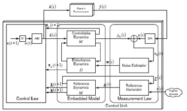
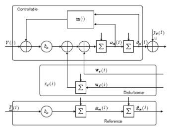
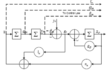
The model error is the key signal in the design process, since it can separate the uncertainty estimation and model-based control design [14]. Model error (11) is also the key signal of the Internal Model Control (IMC) [17]. IMC does not recognize that em(i) can be fed back to the internal model as the source of the past uncertainty. Instead it is fed to the control law which is compelled to be designed in a robust way. A better use of the model error is made by observer-based control systems, for instance ADRC [6] or DOBC [2], where the internal model is completed by a first- order integrator and with input channels where the model error is fed back. The essential scheme of the EMC is presented in Fig. 1 where main components can be identified: a) the controllable dynamics driven by the command vector u(i), b) disturbance dynamics driven by an unpredictable input vector w (i) to be real-time estimated c) the noise/uncertainty estimator [18] and d) the reference dynamics.
3.1. The design model and the embedded model
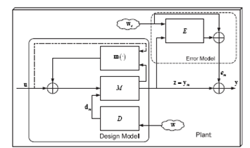
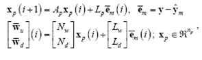
The design model can be represented as a pair of elements as in Fig. 2 the design dynamics and the error dynamics.
For the design dynamics, the state vector x can be partitioned in a controllable part state xc and a disturbance state vector xd , whose dynamics is represented by * and D in Fig. 2. Design dynamics is driven by the command signal u and the noise w .The overall noise can be w
subdivided into, u, the noise entering the controllable states, and w d, the signal driving the disturbance state.
Parametric uncertainty is denoted as a bounded function m (•) defined as
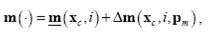 (12)
(12)
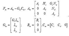
where, m (•) stands for the known information term whereas Δm (•) describes the unknown part, dependent on a bounded parameters vector p m . The last uncertainty in the design model is the neglected dynamics and interconnections denoted with E in Fig. 2. Its output e m together with the model output y m , provides what is expected to be the process output y. According to this the design model can be written as
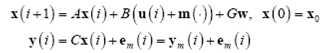 (13)
(13)
where,
 (14)
(14)
with  and
and  . Assume n = nc + nd and ny = nu. No stability assumptions are imposed, the pairs (Ac, Bc) and (A, G) are controllable and pair (A, C) is observable.
The unknown disturbance dynamics is given by
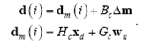 (15)
(15)
The term dm is the response to w and belongs to a signal class D m , which has a forced response that at time i + k, k > 0 is independent of x c (i - h) and u (i - h), h ≥ 0. Term d m may affect any controllable state (it is referred to as non-collocated), whereas the interaction m is collocated.
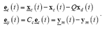
The model error e m is the output of the fractional error dynamics E accounting for neglected dynamics or interconnections. Model error can be written as
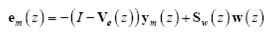 (16)
(16)
3.1.1. The case study
According to the design model in section 0, at least a second order integrator chain must be considered, that is,
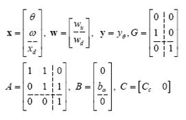 (17)
(17)
The design model block diagram is in Fig. 3. A first order disturbance dynamics has been accounted. The neglected dynamics is due to the electrical part (armature circuit) and the transfer function Ve (z ) in (16) is
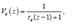 (18)
(18)
where τe = L / RT.
3.2. The embedded model
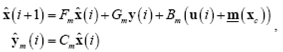
The embedded model makes use of the controllable part and the disturbance dynamics imposed in the design model. Different notations are used for distinguishing between design model and EM. For the EM 'hat' and 'bar' notation is included. 'hat' applies to one-step predicted variables 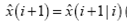 ,'bar' applies to signals which cannot be predicted, e.g., noises. For the EM the parametric uncertainty is set to be only the known component, i.e
  and
em
= 0 is assumed this is,
and
em
= 0 is assumed this is,
 (19)
(19)
Here the EM is considering that the disturbance is absorbing the unknown term associated to Δm, this pose a stability problem and must be taken into account during the design process by the definition of a proper transfer function H (z) defined in [12]. For the case study m (•) is related to the neglected back EMF interconnection thus a discrete time integrator
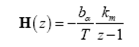 (20)
(20)
The Stability of the entire control loop is guaranteed by the stability conditions introduced in [12], this is,
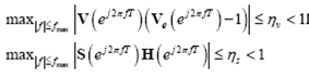 (21)
(21)
3.3. The uncertainty estimator
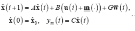
In addition to (17)-(19), the implementation of the EM must be completed with the uncertainty estimator. The general form of the dynamic uncertainty estimator is [18]:
 (22)
(22)
this is, the model e-ror is filtered by the dynamical system  .
.
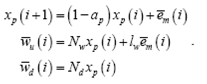
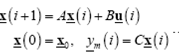
Asymptotic stability conditions are imposed to (22). This transfer function closes the loop with (19), and provides updated estimations of the noises feeding the disturbance dynamics and the controllable states. Then, the overall state prediction equation in compact form is given by
 (23)
(23)
where,
 (24)
(24)
It can be proven that prediction error dynamics reads
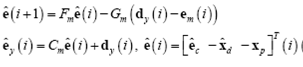 (25)
(25)
with,
 (26)
(26)
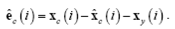
This fact allows the prediction error to be written as a transfer function of uncertain input signals, i.e.,
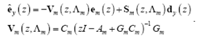 (27)
(27)
Term Λ (Fm) represents the set of eigenvalues of matrix Fm . Equation (27) explains the roles of V m and S m . Here, the larger is the S m bandwidth, the better the estimation of d . On the other hand the shorter is the V m bandwidth, the better the rejection capacity of uncertainty effect on e m . An important result can be established.
The prediction error  in (27) is bounded, if and only if
  is asymptotically stable, i.e.,
  and, Δm and e
m
are bounded. Proof. See [12].
and, Δm and e
m
are bounded. Proof. See [12].
3.3.1. Case study
For the system presented in (17), the uncertainty estimator must be selected to be a dynamic one. This is,
 (28)
(28)
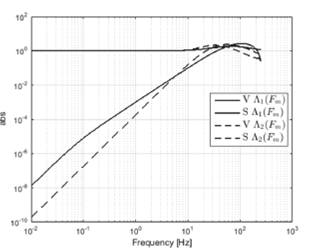
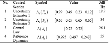
This selection has a physical meaning. The rigid body displacement involves a second order chain of integrators, as said before. However, the input to velocity-position integrator should not include a noise signal as can be seen in Fig. 3. The reason for this is that the derivative relationship between position/velocity is a mathematical abstraction, but physically there is no signal noise affecting this link. The lack of this noise fedback imposes the necessity of considering the dynamic filter X p (t) in (28). Two eigenvalues sets were designed. The first set, Λ1 ( Fm ) is such to guarantee a flat frequency response of the transfer function from reference to measurement. The second set Λ2 ( Fm ) is such to perform better disturbance rejection. Both sets of eigenvalues are in Table 2.
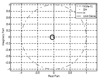
The Fig. 4 show the sennsitivity function Sq and complement function Vq =1- Sq of the state predictor. A BW wider than 15 Hz is necessary to achieve the disturbance rejection performance. For the case study, stability conditions (21) are guarbanteed by a proper selection of the embedded model gain ba. Proof of stability conditions by means of a polar plot is in Fig. 5, where it can be observed how the overall sensitivity S is capable to force H (dashed line) to be inside the unit circle as demanded by (21) that for this study case becomes the more critical stability condition.
3.4. The reference generator
The reference generator or reference dynamics (RD) has the same expression than the EM (19), but free of noise and disturbance dynamics, leaving only the controllable dynamics. The RD only accounts for known terms, i.e.,
 (29)
(29)
Roughly speaking, reference dynamics implements the state trajectories that fulfill input.  Nominal trajectory generation may follow diverse methodologies, linear or nonlinear, closed or open loop, according to what is required for reference tracking, here two methodologies are presented
3.4.1. Closed loop reference generator
For the case study a linear closed loop system is selected, by defining a nominal tracking error 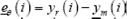 . A simple approach has been followed for trajectories generation, by considering the same structure of the embedded model, without the disturbance dynamics. In order to keep the derivative relationship between position/velocity free of noise a dynamic filter
  is introduced in the same way as in the disturbance estimator
 (30)
(30)
where the state  is included for closed loop stability. The block scheme of the reference generator is presented in Fig. 6.
The frequency response of the reference generator is designed to be as flat as possible within the desired BW. The BW is set at 10 Hz in section 0, which can be achieved by a proper selection of the eigenvalue set Λ(AR) of the closed loop dynamics formed by the combination of (29)-(30). The signal to be tracked by the closed loop is the one provided by this system, i.e., the pair  given nominal command
  .
.
3.4.2. A stepwise guidance as a reference generator.
The reference generator is in charge of computing the EM reference trajectories, these trajectories may be subject to constrains in command or states and must respond to real-time operation requests. It can cope with common control problems like not uniform overshoot in controllers subjected to stepwise user operation requests and persistent excitations typical in industrial applications [19]. By the inclusion of command profile defined as
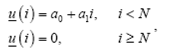 (31)
(31)
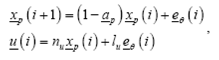
where the coefficients are selected to guarantee the desired settling time N (command saturation dependent) and desired EM states values by using the following closed form solution
 (32)
(32)
3.5. The control law
The control law aims to provide the performance to the control loop. Define the 'true' tracking error as the reference minus the design variables, this is
 (33)
(33)
The ideal stabilizing control law is given by
 (34)
(34)
The control law (34) includes disturbance cancelation terms and it is called ideal since it is able to reject disturbance d in (15) with the exception of the noise. Disturbance x d has been included in error (33) with the objective of non-collocated disturbance cancelation.
Assume w is bounded and zero mean. The tracking error (33) is bounded and the mean value tends to zero with control law (34) if and only if the Davison-Francis relationship
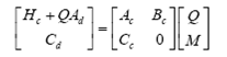 (35)
(35)
Has a solution and the matrix  is asymptotically stable, with eigenvalues set
  . Proof. See [12].
3.5.1. Case study
From (17) and (35) disturbance compensation matrices can be easily found by solving
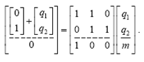 (36)
(36)
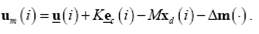
Then, Q = [0 0]T and m = 1. After replacing these parameters and by considering gain matrix K = [ kθ kω ], the control law can be written as
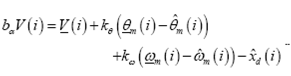 (37)
(37)
There is no room for a complete development of an EMC design that guarantees stability and disturbance rejection performance based on (27) and (21). Eigenvalues obtained from that process for control parameters in former case study sections 0, 0 and 0 are summarized in Table 2.
4. PID design
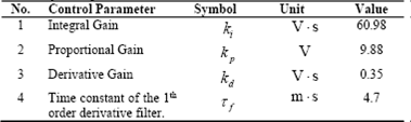
The PID was designed using Matlab® PIDtool tuning application. A typical parallel PIDF (a PID with first-order filter on derivative term) control was implemented, always keeping in mind the desired control performance. The PID parameters and are summarized in Table 3.
5. Experimental results
Experimental results aim to verify the requirements imposed in (8)-(10) are fulfilled. The control algorithms were implemented by using QUARC® real time control software.
5.1. Time responses
5.1.1. Slew rate
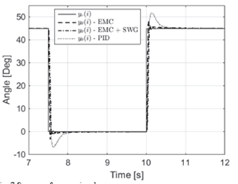
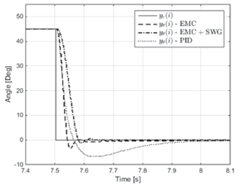
The slew rate was tested through a square-wave reference position. An angular displacement of n4 (45°) was used. The Fig. 7 shows the position reference, a 0.2 Hz square wave, denoted with a continuous line; the measured angular position response is depicted with a dashed line for the EMC, a dash-dotted for EMC with the stepwise guidance (SWG), and a dotted line for the PID. The Fig. 8 shows the response to a decreasing position jump, which requires a negative voltage variation. It can be noticed from Fig. 8 the considerable overshoot exhibited by the PID control of around 15%, whereas for the case of EMC the overshoot was reduced to 3% with the inclusion of the SWG. The settling time for the EMC is around 80ms while the PID exhibit a settling time around 420ms.
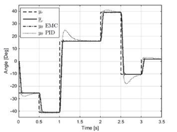
The performance of the EMC controller by considering the reference generator for stepwise operation request is presented in Fig. 9. The measured angular position is depicted with a dash-dotted line for the EMC and dotted line for the PID, while the operation request
yr (i
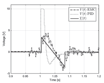
) and reference trajectory  are presented in dashed and solid line respectively? It can be noticed that the non-uniform overshot exhibit by the PID controller, is not present in the EMC as expected due to the inclusion of the reference command (31) In Fig. 10 an enlargement of the voltage control law around 1s is presented for both controllers. It can be observed that the PID controller shows a command saturation. This behavior explains the non- uniform overshoot presented in the measured angular positions in Fig. 7-10. It is also presented in solid line the reference command
  for the EMC control law in (34) for disturbance/uncertainties compensation, the closed loop term can also be appreciated.
5.1.2. Time delay and tracking
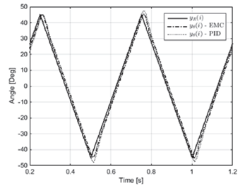
The time response to a 2 Hz triangular external input is shown in Fig. 11. Here an angular displacement of π/4 (45°) was used, it can be seen that time delay of the measured angle (denoted with dash-dotted line) with respect to external reference (continuous line) is smaller than 20 ms, as required in section 0. Same can be said for PID response (dotted line) but an overshoot when there is a change of sign in the derivative is observed.
The Fig. 13 shows the tracking errors for the case of triangular input, in this figure can be appreciated the effect of the overshoot already mentioned. Theoretically, this tracking error must be close to a square-shaped signal. However, the error reported for the case of PID controller shows the spikes produced by the time trajectory overshoot. The residual tracking error  is shown as a dotted line, presenting the distance between the nominal error and the measurement.
Source: The authors
Fig. 9 Performance of the controllers with stepwise operation request and persistent excitation.
Source: The authors
Fig. 10 Actual motor command of the controllers with stepwise operation request and persisted excitation
5.1.3. Disturbance rejection
Here a constant reference of 45° was introduced, but in this case disturbance rejection properties are analyzed. An external torque disturbance was electrically added by means of an equivalent voltage. The Fig. 13 presents the tirae trajectories of the equivalent disturbance torque
Tl
(coii)inuous line), and the EM disturbance state prediction  . The external disturbance is modelled as a 40 mN step. plus a first-order colored noise introduced at 10 s. The same tests have been applied to a PID controller.
From the sets of eigenvalues 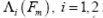 defined in section 0 (see Fig. 4 and Table 2), the first one,
  presents a narrower BW whose disturbance tracking is clearly slower than the perturbation as can be seen in Fig. 13 where the disturbance dynamics X
d (i)
could not track properly the load disturbance which certainly produced a performance degradation in the tracking errors as reported in Fig. 14. Dashed line of Fig. 14 shows the tracking error for this setup; after the introduction of the disturbance, the system tried to bring the error to zero, but it takes a longer time in comparison with the same situation for the PID case. However, when
presents a narrower BW whose disturbance tracking is clearly slower than the perturbation as can be seen in Fig. 13 where the disturbance dynamics X
d (i)
could not track properly the load disturbance which certainly produced a performance degradation in the tracking errors as reported in Fig. 14. Dashed line of Fig. 14 shows the tracking error for this setup; after the introduction of the disturbance, the system tried to bring the error to zero, but it takes a longer time in comparison with the same situation for the PID case. However, when  reaches zero mean its standard deviation remains lower than that of the PID as expected by the difference in the low frequency sensitivity slope.
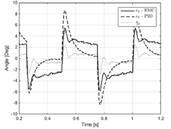
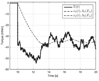
The second set  performs better in term of disturbance rejection that the others controllers according to time trajectories in Fig. 13 this set is able to track the external disturbance properly by producing an almost instantaneous zero mean tracking error.
5.2. Frequency domain analysis
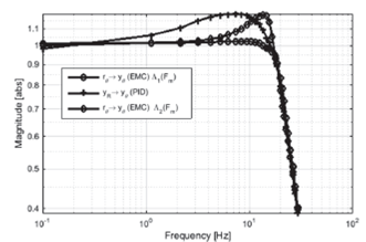
As a complement to performance analysis and in order to verify the initial requirements, additional frequency tests were carried out. The Fig. 15 presents the harmonic responses of the closed loop system. Here the EMC system responses for both sets of eigenvalues are presented and compared with that of the PID controller.
First of all, the PID transfer function (plus-marker line in Fig. 15) presents a considerable overshoot along a wide range of frequencies. This frequency overshoot explains the spike observed in the tracking error in Fig. 14. On the other hand, there are the two sets of eigenvalues of the EMC. The narrower set transfer function (circle-marker line) presents a flat frequency response presented in Fig. 15. For the second case, i.e., a wider BW produced a transfer function with an overshoot. This poses a performance trade-off to be considered, because a flat reference-to-measurement frequency response is always desirable, but it can be obtained at expenses of a poor disturbance rejection capability.
Source: The authors.
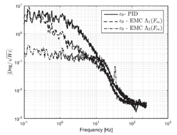
Fig. 16 Power Spectral Density of the tracking error for both control systems and diverse eigenvalues EMC
The PSD of the resulting tracking errors is presented in Fig. 16. It can be noticed that the difference between the rejection factors within the BW is proportional to the difference between the low frequency slopes of sensitivity functions for both controllers as expected.
6. Conclusions
Two types of controllers have been presented in this paper, for the EMC controller an end-to-end design has been outlined and the performance conditions have been exposed and verified. Performance limits due to model/process limitations have been exposed with examples that put in evidence how performance is gracefully improved as a consequence of the inclusion of a parameter free model (the EM) capable of reproduce the behavior of the process and separate model uncertainty through the noise estimator. Further research must be conducted related to the optimal eigenvalues selection, since a trade-off between disturbance rejection and frequency domain characteristics has been evidenced.

