


 Inglês (pdf)
 Artigo em XML
 Referências do artigo
 Enviar este artigo por email
 Citado por SciELO
  Citado por Google
  Similares em
SciELO
Similares em
SciELO  Similares em Google
 Permalink
1. Introduction
Despite the incredible development of electronics that in turn drives the creation of new analytical instrumentation for measurement purposes, it still turns out to be not only costly to perform certain measurements, but in some cases, an arduous task such as, for example, in the characterization of orthotropic materials, [1]. By definition, an orthotropic material is known as one in which its properties, whether for example mechanical or thermal, are unique and independent in their three perpendicular unitary spatial axes i ; 𝑗 ; 𝑘 . That is, the magnitude of its properties or some of them depends on the direction in which it is measured. This characteristic imparts certain properties to the material that make it unique and is reserved for very specific applications. Examples of these are polycrystalline metals, composite polymeric materials, graphite fibers, wood, among others. Given this property, it is very difficult in some situations to experimentally measure the variation of, for example, its electrical or thermal conductivity in those three coordinate axes. Therefore, there are some proposals in the literature to solve this difficulty, one of them being the approach and solution of an inverse problem that proved to be very effective in this situation, [2-5]. Regarding the approach and solution of the inverse problems, it is worth mentioning that its versatility and usefulness are well known in situations where experimentation is limited by obstacles such as high costs of the required instrumentation, and complexity in the realization and direct interpretation of its results, mainly. For the case presented in this article, the problem of heat transfer in a solid is a cause and effect relationship. The causes are determined by the initial conditions, the boundary conditions, the thermodynamic properties, the sources of internal generation and the geometry of the body. On the other hand, the effects are related to the profile of temperature and heat flow in the solid. Therefore, the inverse problem is a powerful conceptual tool that allows linking the mathematical model (cause) with the experimental data (effect). Moreover, this has allowed to address problems and propose solutions that were previously virtually impossible to obtain as, for example: the study of the interior of the earth without the need for expensive drilling, estimating heat transfer coefficients in highly aggressive processes for conventional instrumentation, such as the presence of high intensity electromagnetic fields, measure temperatures in inaccessible places even for the modern instrumentation that is available today, process complex images in astronomy, in computerized tomography for medical analysis, and in many others that it is impossible to number, [6-26]. In all these cases, the strategy used is to solve the problem directly analytically or numerically and solve the inverse problem associated with it. From an analysis of the literature on the subject, it can be seen that conventional methods of local optimization were initially used, such as, for example, the Levenberg-Marquardt method that requires knowing the derivatives of the objective situation function that requires the continuity of the function and stocks of these derivatives. Over time, global optimization strategies appeared that allow obtaining optimal values through a heuristic approach. Again, recent literature is abundant in examples of its use in the solution of inverse problems.
In the present article, the Cuckoo Search Algorithm (ABC) and the Levenberg-Marquardt (LM) Search Algorithm, as well as its hybrid (HCLM), are used to solve the inverse problem that concerns us. The main objective of this work is to estimate the thermal conductivity in an orthotropic material. A couple of numerical solutions are presented as an illustrative example of this strategy. This article summarizes below some relevant concepts about the mathematical model and its solution, together with the description of the optimization algorithms ABC, LM and HCLM. Then, the approach of the direct and inverse problem is presented. It is followed later, compiling the results of the simulations and finalized, with some of the most relevant conclusions.
2. Fundamentals
In this section the optimization algorithms are described very succinctly. In the same way, the objective of the direct problem is established. Then the mathematical model of the conduction heat transfer process that happens inside the solid and its analytical solution is stated. Then, the objective of the inverse problem is established. And in the final part, the objective function to be solved is defined.
2.1. Optimization algorithms
Global optimization is a part of mathematics aimed at finding the extremes of a function in its domain. Within this global optimization there is a generic classification related to the structure of the algorithms, which arbitrarily calls them deterministic and stochastic. In the first are those algorithms that for the same input necessarily produce the same output. In the second, it is characterized because its algorithms depend on randomness, that is, variables or stochastic (random) parameters are present within its components. The deterministic method (LM), the metaheuristic (ABC), and the hybrid of these two (HCLM), which were used, are described below.
2.1.1. Levenberg-Marquardt Method (LM)
The LM is a traditional deterministic algorithm, widely used to solve problems of non-linear characteristics. This method results from the combination of the gradient descent minimization and the Gauss-Newton methods [27]. In this algorithm, when the parameters are far from their optimal value, it acts more like the gradient minimization method. But when they are close to their optimal value, it acts more like the Gauss-Newton method, which makes it easier to determine the desired parameters. Given its wide dissemination in the literature [3], we will not go into greater detail here.
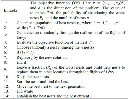
2.1.2. Cuckoo search algorithm (ABC)
This global optimization algorithm was proposed in 2009 by Xin-She Yang and Suash Deb [28], who relied on the behavior of the bird species, the cuckoos and their aggressive breeding strategy. This is related to the way in which these birds deposit their eggs in nests of other species. Such eggs will have a probability 𝑃 𝑎 of being discovered by the "host" birds and not survive. To increase this probability, some species of female cuckoos have managed to perfect the mimetization and posture of their eggs with those of the host species. For the selection of these nests, the cuckoos explore their surroundings using Lévy flights, that is, a small part of the new nests are generated around the best nest found so far. While the other part are generated far enough away from this to avoid being in a non-optimal nest. This algorithm is based on the following rules: The first one says that each cuckoo places one egg at a time and selects a random host nest where it will deposit it. The second says that the nests with the eggs in better quality, will pass to the next generation. And the third part of the assumption that the number of available host
nests is fixed and that the host bird can discover the egg left by a cuckoo with a probability 𝑃 𝑎 (in the interval between [0, 1]). In this case, the host bird can throw the egg at a great distance or leave the nest in order to build a new one in another place. These abandoned nests are replaced by new nests (with new solutions in new random locations). Based on these three rules, the ABC steps are summarized in Table 1. From this table it can be seen that the algorithm requires few input parameters for its execution. These are, the objective function, the initial population 𝑛, the probability 𝑃 𝑎 and the search limits.
2.1.3. Hybrid algorithm (HCLM)
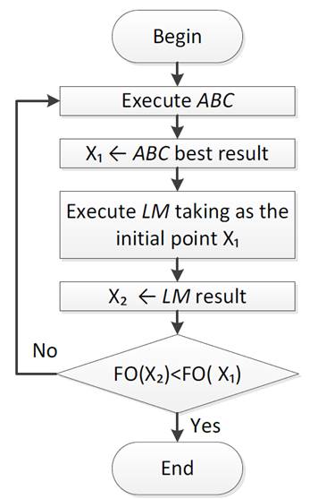
The proposed hybrid algorithm combines the main characteristic of LM (better precision) with that of ABC (greater search space), in order to design a global algorithm that adopts the qualities of its two individual components. This is because the LM is deterministic by nature and if it is provided with initial values sufficiently close to the optimum, it will always find it. On the other hand, ABC is random in nature and finds the optimum in a short time (repetitions), but there is a different success to failure relationship for each run. Thus, the ABC improves efficiency, as well as, accuracy and precision. Fig. 1 shows the behavior of the HCLM. It is emphasized that its topology (serial) is such that the best ABC results become the initial conditions of search for the LM.
2.2. Objective of the direct problem
Determine the transient internal temperature profile in the solid orthotropic material with a defined geometry (rectangular parallelepiped), which is initially at a uniform temperature 𝑇 0 =0. A uniform heat flux is applied to the material in each of the surfaces for 𝑥=𝑎, 𝑦=𝑏 and 𝑧=𝑐, in such a way that there is heat transfer by conduction to the interior of the latter. In addition, it is established that the other three surfaces are thermally insulated. The dimensionless mathematical model is presented in equation (1) where, 𝐾 𝑥 , 𝐾 𝑦 and 𝐾 𝑧 are the respective components of the thermal conductivity in the directions of the unit Cartesian axes, [3]. 𝑇 is the absolute temperature, 𝑡 is the time and 𝑞 𝑥 , 𝑞 𝑦 and 𝑞 𝑧 are the uniform flows of heat of entry in each direction.
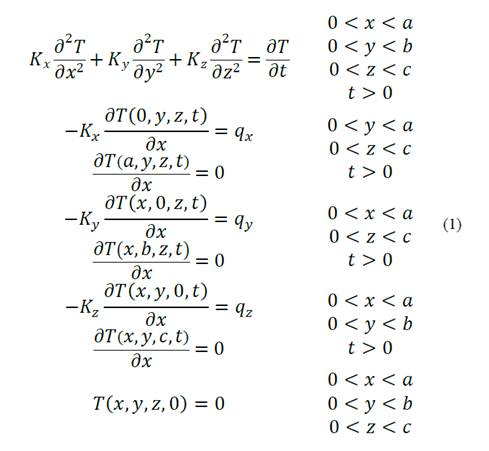
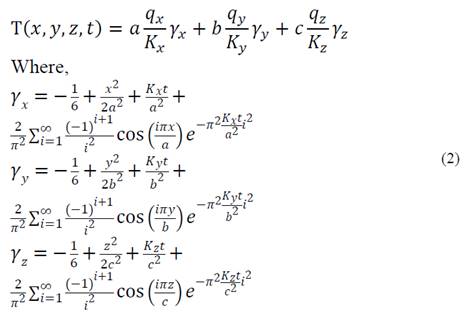
To solve the direct problem, the three components of the thermal conductivity, the geometry of the solid and the initial and border conditions were assumed as known and with sufficient precision in their measurement. The solution of the direct problem, that is, of the mathematical model of the process, is shown in equation (2), [3].
2.3. Objective of the inverse problem
To determine the coefficients of the three thermal conductivities 𝐾 𝑥 , 𝐾 𝑦 and 𝐾 𝑧 , in an orthotropic material with defined geometry (rectangular parallelepiped), assuming known the measured temperature profile within the solid, together with the other parameters of the model, all of them with sufficient precision. To estimate these coefficients, the aforementioned global optimization algorithms were used.
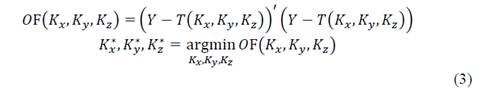
2.4. Objective function
The objective function is the standard L2 squared which is shown in equation (3), where 𝑌 are the measured temperatures, and 𝑇 is the temperature estimated by the model of equation (2). In this work two options were taken as measured temperatures. The first was simply to take the theoretical temperature profile which is obtained by solving the direct problem. On the other hand, the second option was to add Gaussian noise to the theoretical temperature profile to emulate possible sensor errors in the measurement.
Restricted to

3. Results and analysis
In this section, some of the results are first shown using the ABC algorithm in preliminary tests, then, the conductivities of an orthotropic material are found using the LM, ABC and HCLM algorithms and finally an analysis of the obtained results is made.
3.1. Preliminary tests with the ABC algorithm
In this part, two tests were performed on the ABC algorithm. In the first, classic global optimization functions were used in order to verify the correct functioning of the algorithm and in the second, the objective function defined in equation (3) was used to see how it behaves before a spectrum of values of the thermal conductivity.
3.1.1. Test functions
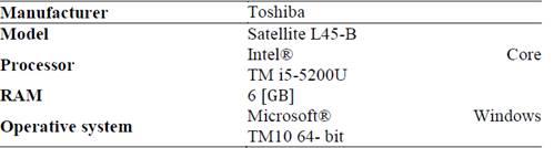
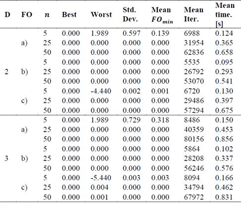
This section shows the verification of the ABC algorithm through the solution of classic optimization functions (FO) such as a) Rastrigin, b) De Jong and c) Griewank. To do this, an algorithm analysis was performed with different population sizes (i.e., 𝑛 = 5, 25 y 50) in two and three dimensions (𝐷). Each configuration was executed 50 times. The specifications of the computer used to perform the tests are shown in Table 2.
The results obtained such as the best solution, the worst, the standard deviation of the solutions, the average value of the objective function, the average iterations used by the algorithm and the computational time of execution, are shown in Table 3. From this, it can be seen that increasing the population improves the search results. However, the use of computational resources also increases.
3.1.2. Objective function
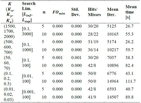
In this section, preliminary tests of the algorithm with the objective function were performed. For this, the temperature profiles were found by varying the components (𝐾 𝑥 , 𝐾 𝑦 , 𝐾 𝑧 ) (the other parameters of equation (2) are shown below in Table 5). Then, the algorithm ABC was executed by varying the population of cuckoos (𝑛 = 5 𝑦 𝑛 = 10). These results are summarized in Table 4, which includes parameters such as the search limits, the minimum value of the objective function, its standard deviation, the number of hits and misses, the average of iterations and the average execution time of the ABC algorithm. The criterion for selecting the correct and incorrect results was directly related to the search range used to find the thermal conductivities and therefore was not fixed during all the tests.
Table 4 Results of the algorithm varying the population of cuckoos and the conductivities.
Source: The authors.
This table shows a hit rate of more than 82% for values of thermal conductivity less than 50. On the contrary, when increasing this conductivity value the hit rate starts to deteriorate up to 56%. A slight improvement in the results is also observed when increasing the population of cuckoos in the algorithm. These results demonstrate the need to combine stochastic and deterministic algorithms, generating hybrids that highlight the positive characteristics of each of their predecessors, as discussed below.
3.2. Estimation of thermal conductivities
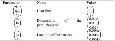
Next, the behavior of the three algorithms for different situations will be analyzed. For this, the results obtained by finding the thermal conductivities are compared by solving the inverse problem, using ABC, HCLM and the LM method. In the first case the values of the thermal conductivities proposed in [3] ( 𝐾 𝑥 = 1, 𝐾 𝑦 = 2 y 𝐾 𝑧 = 3). Moreover, in the second case, the thermal conductivities for crystalline silicon proposed in [30] ( 𝐾 𝑥 = 1.3, 𝐾 𝑦 = 1.46, y 𝐾 𝑧 = 1.78) will be taken. This element was chosen since it is widely used in the development of elements in electronic engineering such as transistors and solar cells. The other parameters of equation (2) are shown in Table 5.
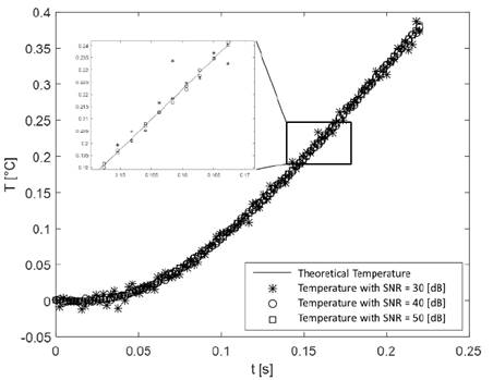
Fig. 2 shows the theoretical temperature profile of the sensor located in (0.004,0.004,0.004) for the case 1 as well as the temperature profile for different signal-to-noise ratios (SNR) (i.e., 30, 40 y 50 [dB]). The graph of the other case was omitted because it is very similar to the one shown. On the other hand, white Gaussian noise was added to the theoretical temperature profile in order to simulate real temperature profiles for cases 1 and 2. According to preliminary results, a SNR of 30 [dB] was defined as the amount of noise minimum allowed to simulate because values below this distort the signal too much.
Source: The authors.
Figure 2 Theoretical and measured temperature profile with SNR = 30, 40 y 50 [dB].
3.2.1. Results of the Levenberg-Marquardt method (LM)
To apply the LM method, preliminary tests were done to find the limits of the initial conditions where it converged and then proceeded to perform the particular tests in each case. As mentioned above, the LM is deterministic so it converges to the same point, as long as the initial conditions are the same. Due to this property, the algorithm was executed once.
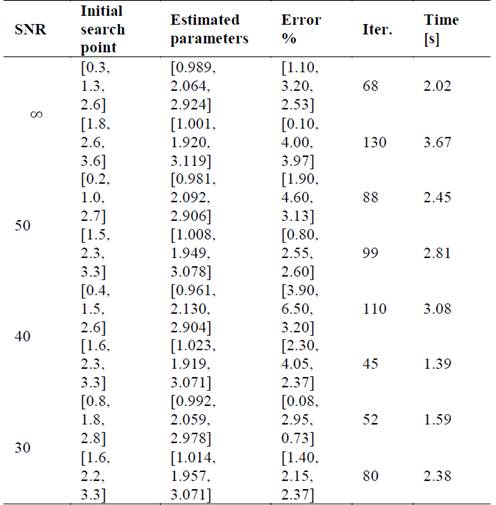
Case 1
Table 6 shows results such as the estimated parameters and the percentage of error obtained by the LM method, as well as the initial search points, the number of iterations and the execution time used. On the other hand, from this table you can see the limited search range to find the thermal conductivities. This evidences a great disadvantage of the LM if some information of the required parameters is not known.
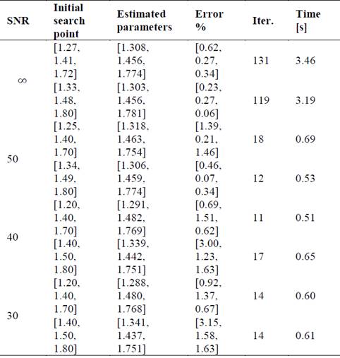
Case 2
Table 7 shows results such as the estimated parameters and the percentage of error obtained by the LM method, as well as the initial search points, the number of iterations and the execution time used. Now, from the results it can be seen that by increasing the noise level (decreasing the SNR), errors increase. This is due to the low quality of the data at small SNR. On the other hand, it is important to note that just as in case 1, there is a limited search range to find the thermal conductivities and that, in addition, this range suffers a reduction compared to case 1 because the thermal conductivities to be found have a greater proximity between them.
3.2.2. Results with the cuckoo search algorithm
As indicated in section 3.1, the ABC presents a good performance with a population of cuckoos equal to or greater than five (𝑛≥5). Therefore, that population size of cuckoos was chosen to implement the algorithm. To verify the reliability of the results, the tests were repeated 50 times.
Case 1
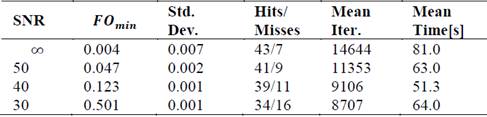
Table 8 shows the results such as the minimum value of the objective function, its standard deviation, the number of hits and misses, the average of iterations and the average execution time of the ABC algorithm. On the other hand, an acceptable performance can be observed in the rate of successes and failures for the four tests carried out. As expected, when the perturbations increase (decrease the SNR) in the temperature profile, the ABC begins to lose precision in the results. It is important to note that those estimated values that differed with the expected values in 0.5 were considered correct and that the search range for each variable is in the range of 0.1 to 100.
Case 2
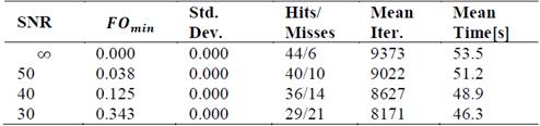
Table 9 shows the results such as the minimum value of the function objective, its standard deviation, the number of hits and misses, the average of iterations and the average execution time of the ABC algorithm. As in the previous case, when the perturbations increase, the algorithm deteriorates in the results. It is important to highlight that those estimated values that differed with the expected values in 0.2 were considered correct and that the search range for each variable is in the range of 0.1 to 100.
3.2.3. Results with the hybrid method (HCLM)
For the hybrid method, the same parameters were used of the ABC and the first two cases were analyzed.
Case 1
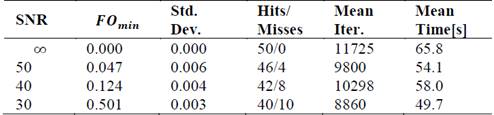
Table 10 shows the results such as the minimum value of the objective function, its standard deviation, the number of hits and misses, the average iterations and the average execution time of the algorithm HCLM. It is important to note that those estimated values that differed with the expected values in 0.5 were considered to be correct. On the other hand, the search range was performed in the range of 0.1 to 100 of each variable. Now, from this table it can be seen that the success rate improves compared to the ABC by 12% if the worst results are compared, which indicates a greater precision of the method to find the required variables. Finally, there is a slight decrease in the execution time, as well as the iterations used if compared with the ABC.
Case 2
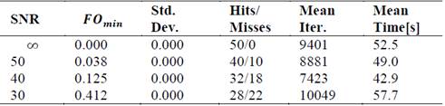
Table 11 shows the results such as the minimum value of the objective function, its standard deviation, the number of hits and misses, the average of iterations and the average execution time of the HCLM algorithm. In this, it can be seen that the success rate improves slightly with respect to the results obtained in case 2 with ABC. We consider that this is due to the noise level of the data used to solve the inverse problem, which does not allow the desired parameters to be reached. Finally, a similar behavior is observed both in the time of convergence and in the number of iterations, in the previous case.
Finally, from the simulations carried out, it can be seen from Tables 6, 8 and 10, that the time of convergence of LM was lower compared to the other two algorithms (ABC and HCLM). One of the factors that influenced this was the search range, since being higher for ABC and HCLM (between 0.1 to 100) compared to LM (0.2 to 3.6), it required more iterations and therefore more computation time. On the other hand, it is observed that the HCLM presents in general a lower number of iterations in comparison with the ABC. This is mainly due to the nature of the hybrid algorithm that takes advantage of the fact that ABC provides LM (as seen in Fig. 1) an optimal starting point, so it does not require many additional iterations to find the optimal global. Similarly, it stands out from Tables 7, 9 and 11, as in the first case, the time of convergence of LM was lower compared to the other two algorithms (ABC and HCLM). This was mainly due to the search range, since being higher for ABC and HCLM (between 0.1 to 100) compared to LM (1.2 to 1.8), it required more iterations and therefore more computational time.
4. Conclusions
This article describes an alternative way of estimating properties such as thermal conductivity in orthotropic materials. For this, the mathematical model that defines the internal temperature profile was used, when the material is subjected to a conduction heat transfer process. Next, the respective inverse problem was defined, which was solved by the cuckoo search algorithm, the Levenberg-Marquardt method and a new hybrid of the latter two. When contrasting the results of the simulations with these three algorithms, it was found that all were able to find the solution, that is, the thermal conductivities for the three orthogonal directions. However, the hybrid has a lower number of iterations and in some cases better execution time when compared to the ABC. We believe that this is due to the presence of the LM. On the other hand, when compared with both, the hybrid algorithm presented a better performance in terms of execution time and number of iterations in most cases. In addition, the solutions turned out to be more precise, even though the search rank was equal to the ABC. Similarly, it was observed that the consumption of computational resources is lower in the LM algorithm. Remember that this traditional deterministic method has the limitation of having to know in advance a region close to the optimal solution, or the probability of not finding it will increase markedly. Thus, we can conclude that for the problem addressed in this work, it is very advantageous to use the new hybrid HCLM algorithm. It is important to highlight that the HCLM can be applied in other fields of engineering as long as the objective function is defined. Readers who wish to follow this methodology, should perform preliminary tests to choose the internal parameters of the algorithm according to each particular application, to obtain better results.

