


 Inglês (pdf)
 Artigo em XML
 Referências do artigo
 Enviar este artigo por email
 Citado por SciELO
  Citado por Google
  Similares em
SciELO
Similares em
SciELO  Similares em Google
 Permalink
1. Introduction
Biomechanical researches strongly rely on accurate force measurements to provide reliable studies and outstanding developments: ground reaction forces occurring during gait analysis and gripping forces occurring during object manipulation are only some applications that demand non-invasive and accurate force measurements.
Inertia and position readings are also demanded in biomechanical studies; with the added complexity that the employed transducers must be installed with minimal interference on the human or animal under study in order to avoid discomfort during motion, consequently, the sensors in Biomechanical studies must be either low profile or such variables must be remotely tracked when possible [1, 2].
Performing accurate position and inertia readings has been practically resolved through the usage of encoders, resolvers and Inertial Measuring Units (IMUs). However, if such sensors result too bulky, high-speed cameras can be used instead [3]. However, performing accurate force readings has always been a difficult task in biomechanical studies because force, unlike position, cannot be remotely tracked.
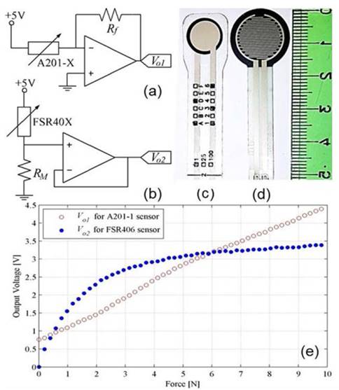
Force Sensing Resistors (FSRs) are cost-affordable force sensors that can be easily integrated into multiple Biomechanical applications [4-6]. Nonetheless, the main reasons for its widespread usage are their low profile and low weight, which are highly desirable characteristics when attempting to perform non-invasive force measurements [6]. Another reason for their wide acceptance is the simple interface circuit required to read sensor’s output, e.g.: voltage dividers or inverting amplifiers. When using an inverting amplifier, see Fig. 1a, an estimation of sensor’s conductance ( 1/Rs ) is obtained through output voltage ( Vo1 ). Conversely, when using a voltage divider, see Fig. 1b, sensor’s resistance ( Rs ) is measured through Vo2 .
Source: The authors.
Figure 1 Driving circuits for: (a) FlexiForce A201-X, (b) Interlink FSR40X. Pictures of: (c) A201-1 and (d) FSR402 next to a ruler in centimeters. (e) Typical sensors’ response: A201-1 (circle red) and FSR406 (solid blue).
Commercially available FSRs can be found on different shapes and nominal ranges: round (FSR400 and FSR402) and squared (FSR406 and FSR408) FSRs are manufactured by Interlink Electronics, Camarillo, CA [7]. Tekscan Inc. from South Boston, MA, offers round (A201-1, A201-25 and A201-100) and several customizable FSRs in his product catalog [8], see Fig. 1c and Fig. 1d. Unfortunately, the overall performance of FSRs is poor compared to well-established force sensing solutions such as load cells and strain gauges. Previous works from Lebosse [9], Hollinger [10] and Komi [11] present a comprehensive review on FSR limitations. Hysteresis and drift are typically one or two orders of magnitude greater in FSRs than in load cells. These conditions are the main drawbacks for the extensive usage of FSRs in industrial and research applications, but a great effort is currently placed on improving their performance.
One trend, within FSR research, is to model sensors’ response with the aim of compensating hysteresis and drift. Relevant works on this scope have been developed by Lebosse [9], Schofield [5], Dabling [12], Vecchi [13] and Urban [14]. Likewise, authors’ previous work has demonstrated that the A201 sensors, working on the piezoresistive principle, are also capable of exhibiting a piezocapacitive response. Different methods were proposed and evaluated by the authors to combine Capacitance ( Cs ) and Conductance ( Vo1 ) readings with the aim of increasing FSR accuracy under static loading [15, 16]. It must be noted that DC/AC voltages were alternately applied to the FSRs to read Vo1 and Cs respectively, followed by a feedforward neural network to optimally combine Vo1 and Cs readings. When compared to the purely conductance model of Fig. 1e [8], a 64% reduction in the force Mean Squared Error (MSE) was obtained. The reduction in the MSE was done at the price of increasing the complexity of the driving circuit which may result prohibitive for certain applications with power or space constraints.
By modeling FSR’s hysteresis through the Preisach operator [17], an improved algorithm for estimating applied forces is here presented. The algorithm only requires conductance readings form the sensor, and thus, the simple driving circuit of Fig. 1a is needed, or Fig. 1b when using Interlink sensors. A considerably computational effort is required to run the inverse Preisach algorithm, but such an effort is justified when the force MSE is dramatically reduced. In order to obtain a valid generalization of results, a total of sixteen A201-1 FlexiForce sensors are used; this sensor matches the required force range (4.5N) of biomechanical applications involving grip and grasp operations. Nonetheless, the methods henceforth discussed are applicable to other models of FSRs.
This paper is organized as follows: Section II describes the experimental setup for gathering sensor data. Later in Section III, experimental data from the sixteen A201-1 sensors are presented with statistics regarding hysteresis. A brief description of the Preisach Operator and its inverse are also available on Section III. Later in Section IV, grip force profiles are exerted on the A201-1 sensors and the inverse Preisach algorithm is tested and compared with the traditional conductance model. In Section V, a generalized sensor model based on the Preisach Operator is presented, followed by conclusions and future work on Section VI.
2. Experimental Set-Up
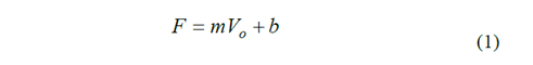
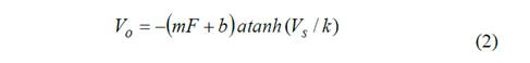
Previous work demonstrated that the A201-X sensors can be electrically modeled as a parallel Rs - Cs device as shown in Fig. 2a [15,16], with Rs exhibiting a hyperbolical dependence on the applied force (F). Since this paper focusses on reducing the force MSE through conductance readings only, capacitance measurements are not henceforth considered. For linearization purposes, conductance variations - measured through Vo1 - have been preferably used in several studies to estimate F [8, 9, 12, 15]; this is possible by inverting the model of Fig. 1e, which yields:
Where m and b are obtained from a least-squares minimization process; the whole procedure is known in literature as sensor characterization and may comprise only increasing or increasing/decreasing forces. It must be noted that the application of either pattern produces a significant effect in m and b values given the hysteresis in the device; this is later exemplified on Section IV. The test bench for sensor characterization and testing comprises electrical and mechanical sensors/actuators as described next.
Source: The authors.
Figure 2 Equivalent model and test bench for characterization of A201-X sensors. (a) Black box model and equivalent circuit for an A201-X FSR. (b) Zoom-in picture depicting the spring (i) for mechanical compliance of the test bench and the bunch of sixteen A201-1 sensors (ii) arranged in a sandwich configuration. (c) Picture of the test bench showing the stepper motor (iii), the LCHD-5 load cell (iv) and the temperature chamber (v).
2.1. Mechanical setup
In order to get a trade-off between nominal force and resolution, a linear stepper motor was accommodated with a spring to exert forces over the bunch of sensors depicted in Fig. 2b. The mechanical compliance of the test bench was modified through the stiff constant of the spring; and the force control loop was closed using data from a high accuracy LCHD-5 load cell with 22N capacity. The set-up could arrange up to sixteen sensors simultaneously with a resolution of 1.4mN and a maximum dF/dt of 22.6N/s. These characteristics were more than enough to emulate force profiles exerted during grip and grasp operations such as those reported by Stolt [18] and Melnyk [19].
The sensors were arranged in a sandwich configuration and then placed inside a temperature chamber that held operating temperature at 25ºC±1ºC to avoid undesired effects caused by thermal drift, see Fig 2c. Considering that the main scope of this article is to reduce the force MSE through hysteresis modeling and compensation, it was not embraced the inclusion of changing temperatures as an additional variable. Finally, it must be noted that the sandwich configuration depicted in Fig. 2b added extra weight to the sensors located at the bottom; this condition was taken into account for the linear regression method (1) and the Preisach Operator later described on Sections III, IV.
2.2. Electrical setup
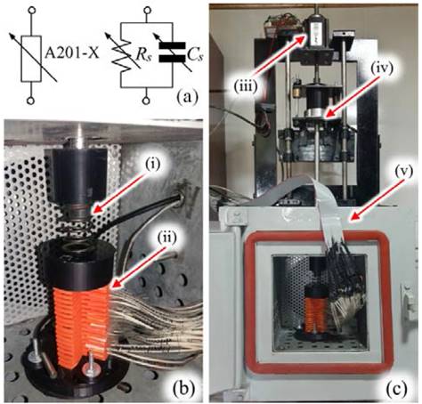
A modified version of the circuit from Fig. 1a was implemented to perform voltage readings in the sixteen sensors, see Fig. 3. A time-multiplexed scheme comprising four analog multiplexers (ADG444) was implemented to readout Vo . The feedback Resistor ( Rf ) was set to 10KΩ and the supply Voltage ( Vs ) was set to -1V.
Source: The authors.
Figure 3 Simplified diagram of the time multiplexed circuit to measure conductance ( Vo ) in sixteen A201-1 sensors, S0 through S15.
It must be remarked that the FlexiForce sensors exhibit a subtle saturation effect in the form of hyperbolic tangent in regard to Vs variations; this avoids that m and b can be recalculated when Vs is changed given that k in (2) changes from one sensor to another [16]. In practice, this implies that (1) is valid only for a constant Vs during sensor operation:
3. Hysteresis characterization, modeling and compensation based on the Preisach operator
3.1. Characterization of hysteresis in FSRs
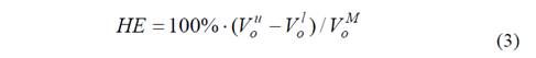
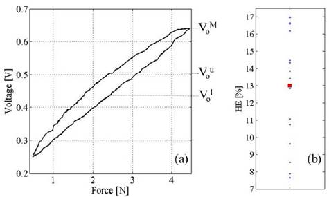
Triangle force profiles of 4.5N were exerted over the sensors to observe Vo during loading and unloading events. Equation (3) was employed to assess the Hysteresis Error (HE) based on the metrics shown on Fig. 4a. Results from the sixteen sensors are represented by data points on Fig. 4b.
Note that hysteresis ranges from 7.6% to 17%, with the maximum Vou - Vol occurring typically at half of the nominal sensor range, such values notably differ from what the sensor manufacturer reports at [8] with HE<4.5%. However, the manufacturer estimates the HE at 80% of the nominal sensor range. Dabling reports in [12] a 7.4% hysteresis for the Tekscan A401-25 sensor, which is consistent with the results from Fig 4b.
Source: The authors.
Figure 4 Hysteresis in the A201-1 sensor. (a) Plot representing the maximum voltage difference between loading ( Vol ) and unloading ( Vou ) events, occurring at the same F. (b) Scatter plot of the HE for sixteen A201-1 sensors. The average HE is shown with a squared red marker.
3.2. Modeling hysteresis through the Preisach operator
In order to compensate for hysteresis, it needs first to be modeled. The Preisach Operator (PO) is a common approach to model hysteresis; it has been successfully employed in nanopositioning applications with piezoelectric and magnetostrictive actuators [17, 20]. An in-depth explanation of the PO theory has not been provided here, but readers may refer to Tan [21] and Visone [17] for such a purpose.
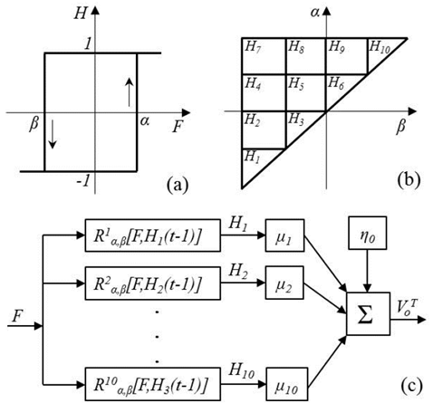
The ability of the Preisach Operator to model hysteresis is next described with an example focused on the A201-1 sensor, where Rα,β[F,H(t-1)] is the delayed relay output represented in Fig. 5a as H and as H(t) in (4). The applied force, F, is the time-varying input.
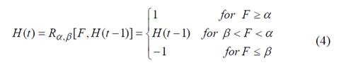
The function Rα,β[F,H(t-1)] is known in literature as the Preisach Operator or Hysteron, where parameters α and β come from the discretization of F into nh levels, summing a total of nq Hysterons:

Source: The authors.
Figure 5 Preisach Operator and elements. (a) Plot of the delayed relay output representing the mathematical function of a Hysteron. (b) Preisach plane with nh=4 and 10 Hysterons. (c) Block diagram representing the totaling function for modeling hysteresis in the A201-1 FSR.
As in Fig. 5b with nh=4 , there is a total of 10 Hysterons ( H1 ~ H10 ). The totaling function ( VoT(t) ) is a discrete function that embraces the contribution from each delayed relay output ( H1~H10 ) weighted by ( μ1~μ10 ) plus an offset ( η0 ); this process is performed on each sampling interval to obtain a discrete model of the sensor hysteresis. A graphical representation of the totaling process is depicted on Fig. 5c.
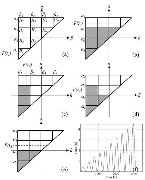
At the beginning of a trial, all of the Hysterons are deactivated, i.e., initialized at y(t-1)=-1, see Fig. 6a; this implies that F(t1) ≤ α1 . As F(t2) increases beyond α3 , Hysterons H1 to H6 , are activated and their relay outputs change from -1 to 1. Active relay outputs are gray colored in Fig. 6a and ahead. Later, the applied force decreases up to F(t3) where F(t3) ≤ β2 , and thus, Hysterons H3 , H5 and H6 are deactivated as shown on Fig. 6c. Finally, in Fig. 6d, force is increased again up to F(t4) and the only Hysteron that changed is H3 since α2<F(t4)<α3.
Source: The authors.
Figure 6 Preisach plane and input signal for hysteresis characterization, active hysterons are gray colored. (a through d) Evolution of the Preisach plane under increasing and decreasing forces with initial condition Ψ0=(H1~H10)=-1 at Fig. 6a. (e) Final Preisach plane for an input force F(t5) with initial condition Ψ0=(H1~H10)=-1. (f) General form of the required input signal for hysteresis characterization.
The ability of the Preisach Operator to model hysteresis is exemplified as follows: let’s say that in a new trail represented in Fig. 6e, the applied force is straight incremented from F(t1) ≤ α1 up to F(t5) , with F(t5)=F(t4). Note that in Fig. 6e the Hysterons H1 to H3 are activated, which differs from the previous memory curve of Fig 6d. Such a difference yields different values on the output totaling function, VoT(t), because of the different trajectories employed to reach F(t4) and F(t5) on each case.
The weight values of each Hysteron, μ1~μ10 , and the offset, η0 , are estimated on an empirical basis, following a characterization process somewhat similar to that recommended by the sensor manufacturer [8]. In a general case with nh levels of discretization, there is a total of nq Hysterons that are grouped in the so-called memory curve (Ψ). The Preisach density function ( μ(α,β) ) is defined as the collection of weights representing the contribution of each
Hysteron to the totaling function, VoT(t) . The function μ(α,β) is nonnegative with a total of nq elements. It must be noted that in order to model hysteresis, a total of nq+1 parameters - μ(α,β) plus η0 - must be estimated through a least-squares minimization process that ensures the nonnegative constraint of the Preisach density function. During characterization, it is important that the input force profile ensures the activation and deactivation of all the Hysterons; by doing this, an appropriate estimation of μ(α,β) and η0 is obtained.
Stakvik presented in [20] a guideline for creating an adequate input signal intended for hysteresis characterization; the signal consists of incremental-amplitude sine waveforms as shown on Fig. 6f. It must be remarked that the hysteresis is a rate independent phenomenon, and thus, the frequency of the input-sine profile does not affect the identification process.
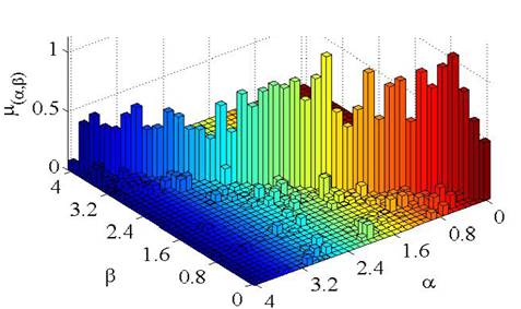
Finally, the identification of μ(α,β) and η0 was carried out by applying a modified version of Fig. 6f. Triangle force profiles were used instead of sines with forty evenly spaced amplitudes starting from 0N up to 4.5N. Likewise, the discretization level was set to nh=40 during the data fitting process that estimated μ(α,β) and η0 . The resulting μ(α,β) is plotted on Fig. 7 for one of the sixteen sensors previously shown on Fig. 2b, similar density functions were obtained for the rest of sensors.
Source: The authors.
Figure 7 Preisach density function for nh=40 , showing the 820 weight values for an A201-1 FlexiForce sensor.
In practice, the maximum value of nh is limited by the Repeatability Error (RE) of the device; typically RE=2.5% for the A201-1 sensor [8]. This implies that the uncertainty in sensor output, Vo , for a given applied force is of 2.5% and thus, the sensor can resolve a maximum of 100/2.5 force intervals without overlapping.
3.3. Compensating hysteresis in FSRs through the inversion of the Preisach operator
When estimating F based on Vo readings, the PO model must be inverted in order to compensate for hysteresis. Unfortunately, an analytical expression for the delayed relay operator cannot be formulated; and thus, an approximate numerical solution must be found instead.
Given the initial conditions: Ψ0 curve with all Hysterons deactivated, (H1~H10)=-1 , and the applied force F0=0N . At the next sampling interval with F1>F0 , the numerical inversion algorithm activates the Hysterons following the same order depicted in Fig. 6, i.e. H1 , H2 - H3 , H4 - H5 - H6 , and so on. The process is repeated until VoT(t) reaches the closest match to the measured voltage V1 at the FSR. The required force to activate the above-cited Hysterons is the approximate numerical solution of the inverse PO model. The procedure is conveniently known in literature as the Closet Match Algorithm (CMA) [21]. The output of the CMA is discrete (F), just as the PO model is. However, a continuous implementation of the CMA has been already developed in [20], but for space constraints, it has not been discussed or implemented here.
4. Experimental results and analysis
Grip force profiles, based on grip data issued from Stolt [18] and Melnyk [19], were exerted on the A201-1 sensors using the experimental set-up previously described on Section II. The performance of the CMA to estimate F was comparatively evaluated with the linear regression model (1), which is the manufacturer recommended method. It must be noted that the linear regression model is the preferred method in research applications [4, 5, 9-13]. Two sets of m and b constants were calculated using the triangle force profiles of Section III.B. The first set of m and b constants used only the increasing data points, whereas the second fit employed the whole data.
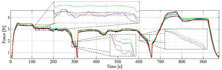
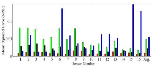
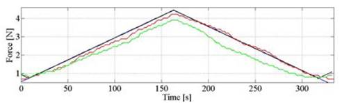
Experimental results for a given sensor are graphed on Fig. 8, together with an error bar plot on Fig. 9 representing the force MSE for the sixteen sensors and the three models, i.e.: the CMA and the two aforesaid linear regressions. In average, the CMA yields a considerable reduction in the MSE compared to the models based on (1), 54% and 76% respectively. The reduction in the force MSE is paid by a larger computation time, which may limit the usability of the CMA in some real-time applications, but if time is not a constraint; the CMA can run off-line and get the best of a FSR. This is the case of most biomechanics researches in which data are collected and later analyzed [4, 5]. However, a fast implementation of the CMA is possible if dedicated hardware is used, i.e., employing FPGA technology [22].
Source: The authors.
Figure 8 Force estimation through different methods: (red) CMA using a sensor-tuned Preisach density function and η0 , linear regressions using increasing data points only (green) and the entire dataset (black). Real force profile based on grip data from Stolt [18] and Melnyk [19] (blue).
Note that the dispersion of the MSE is narrowed when force estimation is done on the CMA (red bars on Fig. 9), this occurs because the remaining MSE is only produced by: the Repeatability Error, RE, and the quantization error derived from the discrete CMA. The contribution of the HE to the MSE is suppressed thanks to the PO modeling and compensation via the CMA. Further reduction of the MSE is possible if a continuous implementation of the CMA is performed, just as Stakvik demonstrated in [20]. This statement can be illustrated from the zoom-in plot at the top of Fig. 8. Note that both linear regressions exhibit a subtle swinging due to Vo variations, nonetheless, such variations are not great enough to change the memory curve Ψ, and consequently, the CMA yields a constant output. The implementation of a continuous CMA can better adapt to subtle Vo variations amid a constant memory curve Ψ, and thus, the force MSE would be further reduced.
Source: The authors.
Figure 9 Error bar plot depicting the force MSE for the sixteen A201-1 sensors operating on the following estimation methods: (red) CMA using a sensor-tuned Preisach density function and η0 , linear regressions using increasing data points only (green) and the entire dataset (black), CMA using the Preisach-scaled parameters, μs(α,β) and ηs0 (blue).
5. Generalized sensor model for hysteresis compensation: an approach
Obtaining μ(α,β) and η0 is not a straightforward procedure; specialized hardware is required and a time consuming characterization must be performed followed by non-trivial programing. Fortunately, it is possible to simplify the characterization process if the parametrization is performed as follows: Given b0 , the output voltage of a FSR at null force, and Vnom , the maximum output voltage at the nominal sensor range; then, the following linear transformation can be applied to any Vo reading during both: the estimation of μ(α,β) and η0 , and later, during sensor operation.

The scaled output voltage ( Vos ) is normalized, just as the resulting Preisach-scaled parameters are, μs(α,β) and ηs0 ; this implies that they can be used to estimate F with hysteresis compensation for any sensor, requiring only the experimental measuring of b0 and Vnom on each new device.
However, it must be pointed out that during sensor operation, the CMA running on the basis of μs(α,β) and ηs0 can compensate for a specific amount of HE, see Fig 4, this implies that if a given sensor exhibits a larger HE than that modeled by μs(α,β) and ηs0 , the resulting F will still exhibit some hysteresis (underfitting case). Conversely, if a given sensor has a lower HE, the resulting F will reflect hysteresis overfitting; both cases are presented on Fig. 10. Hysteresis overfitting is characterized by a time-ahead output during sensor unloading (green data on Fig. 10), especially noticeable around the maximum Vou - Vol which occurs at half of the nominal sensor range, see Fig. 4. Conversely, if hysteresis is under-fitted, the CMA produces a lagged sensor output during the unloading stage (red line on Fig. 10).
Source: The authors.
Figure 10 Triangle force profile (blue) and sensors output response showing hysteresis underfitting (red) and overfitting (green).
The Preisach-scaled parameters were obtained by applying the linear transformation (6) to the data gathered for the sixteen sensors. The resulting μs(α,β) and ηs0 were later used to estimate F using the CMA. The blue error bars of Fig. 9 shows the resulting MSE when using the Preisach-scaled parameters during force estimation. Note that the MSE is higher than that reported on Section IV (individual Preisach parameters tuned for each sensor); this is a logical consequence of hysteresis-overfitting and underfitting. Likewise, mixed results were obtained when comparing to the linear regression methods, indicating that additional work is required on this subject.
6. Conclusion and future work
The Preisach Operator and the Closest Match Algorithm (CMA) have been successfully implemented on sixteen A201-1 sensors to both: model hysteresis and compensate for hysteresis effects during sensor operation. In the latter case, a considerably reduction of 54% was obtained in the force MSE compared with the manufacturer-recommended method based on linear regression. This is an important contribution that narrows the gap between the highly accurate load cells and the low-profile low-cost FSRs. Further MSE reduction is possible by implementing a continuous CMA, this is left as a pending task for future work. It must be remarked that hysteresis modeling and compensation required no-additional hardware during sensor operation, which is a highly desirable characteristic in applications with power or space constraints.
Considering that hysteresis modeling is not a straightforward procedure, a generalized model for hysteresis compensation has been proposed for the A201-1 sensor. However, mixed results were obtained because of hysteresis overfitting and underfitting. Future work is required on the subject in order to develop several Preisach density function focused on compensating for a specific amount of Hysteresis Error. This task can be carried out for sensors exhibiting a linear output, such as the Tekscan A201-X, and for sensors with a nonlinear response, e.g. Interlink FSR40X and Peratech QTC sensors.

