English (pdf)
 Article in xml format
 Article references
 Send this article by e-mail
 Cited by SciELO
  Cited by Google
  Similars in
SciELO
Similars in
SciELO  Similars in Google
 Permalink
1. Introduction
Well testing is the cheapest way of reservoir characterization. Although it provides the most accurate option for finding distances from well to faults/discontinuities, reservoir characteristics and geology speed up or delay the transient wave travel time, leading to erroneous interpretations when isotropic methods are used.
Most of the well test methods to estimate the distance from wells to linear boundaries are presented for isotropic cases. In the semilog plot, a fault is detected when the slope of the radial flow regime doubles its value. The intercept of lines going through these two semilog lines are normally used to find the distance from the well to the fault. Among the isotropic methods, the following can be named: [8,9,17,20], MDH presented by [2,3,6,7,16,18,21,22], Sabet presented by [24] and [24]. [13] compiled the methods produced until 1970.
Regarding the application of the pressure derivative, the work by [4] presented a new mathematical solution for a linear boundary detection, including wellbore storage and skin factor. The authors also developed a type-curve matching procedure and verified its application with a synthetic example. The first TDS Technique, [25], approach to find the distance from the well to a given linear discontinuity was presented by [19]. To estimate fault-to-well distance, they used the time at which radial flow regime ends.
[23] were the first to include fault detection in anisotropic reservoirs. Although they used conventional analysis (intersection of semilog lines) for the interpretation, new expressions for determining actual well image location and true distance were included. Later, [14] and [15], based on the work by [23], developed a new mathematical solution, including wellbore storage and skin factor. They provided both TDS Technique and type-curve matching interpretation techniques. Once the fault distance is found, the true distance-corrected by anisotropy effects-is obtained using the formulae of [23].
This work is also based on the works of [15] and [23]. A more general and practical formula was also developed using the time at which the radial flow regime ends. However, this new formula includes the effects of both anisotropy angle and anisotropy index. It was obtained by creating a unified behavior of pressure derivative against ( FC t D /(I A 0.5 L f 2), where ( FC is a correction factor involving the anisotropy angle and I A is the areal anisotropy index (k x /k y ). When the ending time of the radial flow regime is obscured by noise, the inflection point observed between the two pressure derivative plateaus is used in a similar equation. However, this inflection point is better determined using the maximum point on the second pressure derivative curve. For the case of a constant-pressure boundary, a negative unit slope line is developed. An equation for such a line was empirically (linear regression) obtained, so an arbitrary point read on such a line is used to find the distance from the well to the discontinuity. Also, the intersect of such a line with the extension of the radial flow regime line is used to develop another expression to find the distance to the constant-pressure boundary. Synthetic examples and a field case were used to successfully verify the developed equations. Care must be taken if an anisotropic reservoir is dealt with as an isotropic system, since the error could be as high as 100%.
2. Mathematical model
The classic assumptions used in well test analysis also apply here; this means that, regardless of gravity, a single and slightly compressible fluid with constant viscosity, a homogeneous porous medium and maximum permeability and minimum permeability are oriented in the x and y directions, respectively, the x-y coordinate system can be transformed by changing the scale along each axis:
Thus, I A the anisotropic index or horizontal permeability ratio, is defined by the following:
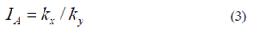
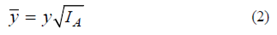
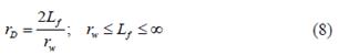
The method of images, [5], can be applied once the coordinate change is achieved to convert to isotropic conditions. [23] presented a general well imaging technique based on Eqs. (1) and (2), so actual image well location is given by the following:
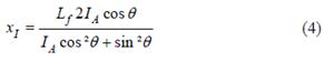
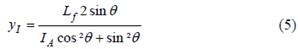
These equations imply that the well image location in an anisotropic medium is a function of both the anisotropy index and the angle formed by the fault and the principal permeability axis. Isotropic system results whenever the fault is normal to either principal axis (( = 0 or (/2) as demonstrated by [23]. Who also provided A better picture is given in Fig. 1, and a detailed development of Eqs. (4) and (5) is presented by [23]. Using these equations, they also arrived at the following:
Source: Authors
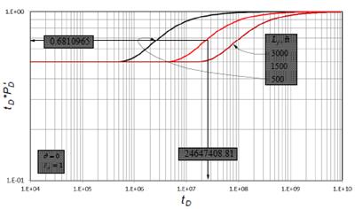
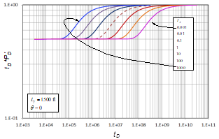
Figure 1 Effect of fault-well distance, L f , on the pressure derivative behavior for isotropic systems
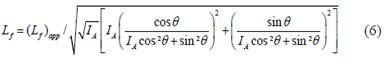
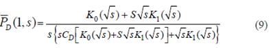
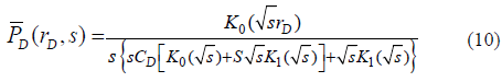
Where (L f ) app is the apparent or uncorrected well-to-fault distance found for the isotropic system case. Estimation of well pressure behavior is obtained once the image well location is determined. The denominator of Eq. (6) can be read from Fig. 9 by [23]. [15] provided a general solution, including wellbore storage and skin factor, for a well near either a sealing fault or a constant-pressure boundary. This solution avoids setting many well images.

Being that
The ( symbol in Eq. (7) considers the solution for either the fault or constant-pressure boundary. When the sign is positive, a sealing fault is near the well. When the sign is negative, a constant-pressure boundary is then set, and radial stabilization characterized by a negative-unit slope in the pressure derivative curve is presented once the constant-pressure boundary is felt by the transient wave. Radial stabilization has been characterized by [11] and [12]. The two terms at the right side of Eq.(7) are defined by the following:
3. Interpretation methodology
The TDS Technique, [25], is a powerful and practical interpretation technique that uses characteristic lines and features found on the pressure derivative plot. The solutions of the diffusivity equation for each individual flow regime are used to develop mathematical expressions to determine reservoir parameters. Maximum points, minimum points and inflection points are also used to develop equations for further reservoir characterization or parameter verification. Even though the intersection of the governing equations of two given flow regimes do not have any physical meaning, its use also allows further expressions to be developed to create more equations.
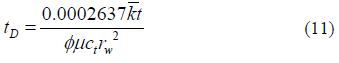
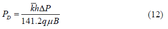
Let us start by defining some dimensional quantities for oil reservoirs:
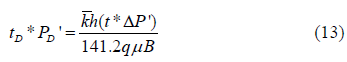
The dimensionless pressure and pressure derivative follow:
The application of Eq.(7) leads to several pressure derivatives versus time behaviors, as displayed in Figs. 2 through 5. As can be seen, a variety of derivatives and, of course, pressure responses are obtained as the parameters are varied. This makes the application of type-curve matching difficult, as proposed by [15]. [15] also extended the TDS Technique for anisotropic systems but they involved an expression for the estimation of the true well-to-discontinuity distance with Eq.(6), presented by [23]. A more practical application of the TDS Technique will be developed here.
Source: Authors
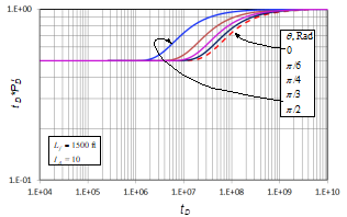
Figure 2 Effect of anisotropy index, I A , on the pressure derivative behavior for anisotropic systems; ( = 0 and L f = 1500 ft.
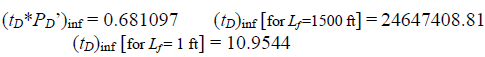
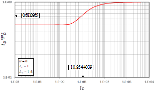
Fig. 1 presents the pressure derivative behavior for three different well-to-fault distances in isotropic systems. A unique behavior for the three systems is required to obtain the characteristic points that will be used to develop the interpretation equations. Notice in Fig. 1 that the dimensionless time at which the fault is felt increases as the well-fault distance increases; then, for the behavior unification, the dimensionless time is divided by the distance, L f n , where n is an unknown exponent that may affect the unified behavior. Although, not shown here, when n = 1, no unified behavior is obtained; then, n must be different than one and ought to be determined. A simple procedure to find n is based on the use of the pressure derivative curve with L f = 1 ft.; in such a case, n has no impact on the pressure derivative curve, since a division by the unity does not cause any alteration on the result (see Fig. 5). To find the value of n, an arbitrary point is chosen during the time between the two plateaus seen on the pressure derivative, which is the matching zone of interest on the curve L f = 1 ft. The arbitrary chosen reference point was the inflection point. An analogous point is taken from another curve with L f > 1. For this case, the arbitrary curve for L f = 1500 ft. was chosen. The reading points are then obtained from Figs. 2 and 6:
Therefore, the following matching expression is given:
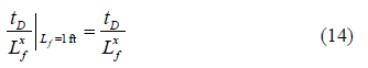
Which can easily be written as
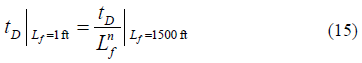
Replacing the reading values from Figs. 2 and 6.
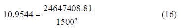
Then, n = 2 is determined using Eq.(16). Therefore, after dividing the dimensionless time of Fig. 1 by L f 2, a unique curve, as given in Fig. 4, will be obtained.
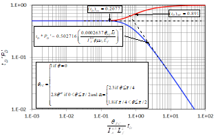
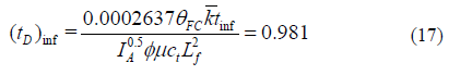
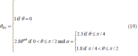
A similar treatment was first performed on Fig. 2 for the anisotropy index. As seen on that plot, the inflection point increases as the anisotropy index increases its effect in the denominator. An n value of 0.5 was found with a procedure similar to the one used for the well-to-fault distance case. In Fig. 3, the effect of the anisotropy angle, (; is presented. As ( increases, the inflection point shows up earlier, meaning that its effect goes in the numerator. The n exponent for this case is the unity, but the effect changes when ( ( (/2. Then, finally, the unified behavior is obtained when the dimensionless time is multiplied by a correction factor, ( FC , and divided by the product of the square root of the anisotropy index times the squared well-to-fault distance. The range of angles applied for ( FC is given in Eq.(19). This also works for the constant-pressure boundary case, as shown in Fig. 4. Fig. 6 presents a unified dimensionless pressure derivative behavior against ( FC t D /(I A 0.5 L f 2). In other words, universal dimensionless pressure derivative behavior is obtained. From that plot, the inflection time, t inf-once the fault has been felt-for all cases is given by the following:
Source: Authors
Figure 3 Effect of anisotropy angle on the pressure derivative behavior for anisotropic systems; I A = 10 and L f = 1500 ft.
Source: Authors
Figure 4 Mixed effect of anisotropy index, I A ; anisotropy angle, (; and discontinuity-well distance, L f , on the pressure derivative behavior for an anisotropic system
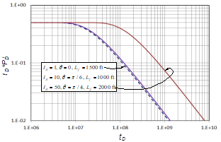
Source: Authors
Figure 6 Unified pressure derivative behavior for anisotropic system with different values of anisotropy index, I A ; anisotropy angle, (; and discontinuity-well distance, L f
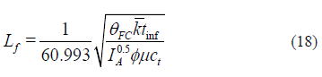
The distance from the well to the linear boundary is obtained from the following:
The anisotropy angle correction factor, ( FC , is given by the below:
For the sealing-fault case, the inflection time is better obtained using the maximum point obtained on the second pressure derivative curve.
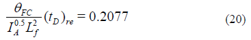
It is also shown in Fig. 6 that the radial flow regime ends at a dimensionless time of 0.2077, meaning
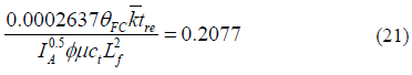
Replacing Eq.(11) in the above equation leads to
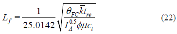
From which the below is developed:
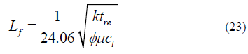
This is very close to the expression given by Guira et al. (2002) for an isotropic case:
As observed in Figs. 5 and 7, the constant-pressure single-boundary case has an especial feature. Radial stabilization develops once the boundary has been reached by the transient wave, and the pressure derivative curve displays a negative unit-slope line. After the unification of the dimensionless pressure derivative curve, the governing equation for such a line obtained from the regression analysis is
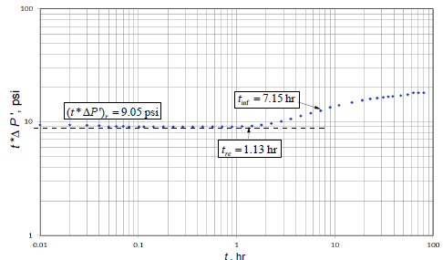
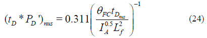
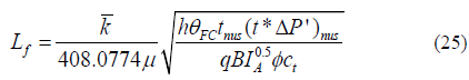
Where rnusi stands for radial negative unit-Slope intersection. Replacing the dimensionless quantities given by Eqs. (11) and (13) in Eq.(24) and solving for the well-to-discontinuity distance yields the following:
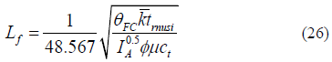
The point of intersection between the radial flow regime line and the radial stabilization negative unit-slope line is a unique feature; by equating the right side of Eq.(24) to one half and solving for the well-to-discontinuity distance, it is obtained:
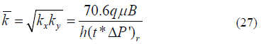
Finally, the reservoir permeability is found from an expression given by Tiab (1995):
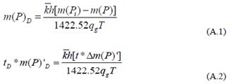
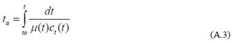
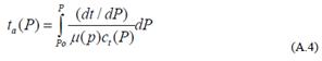
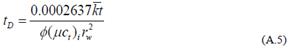
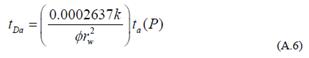
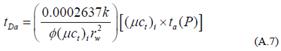
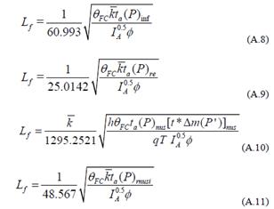
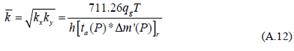
The gas equations are provided in appendix A.
4. Examples
4.1. Synthetic example 1
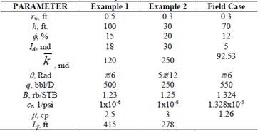
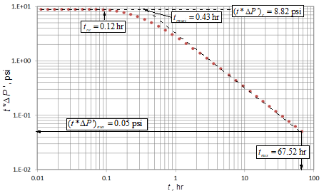
Using the data given in Table 1 and the pressure derivative plot of Fig. 7, find the distance from the well to a sealing fault.
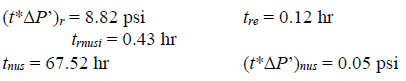
Solution. The following information was read from Fig. 7.
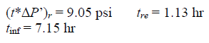
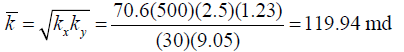
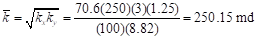
Find reservoir permeability using Eq.(27):
Find the anisotropy angle factor using Eq.(19):
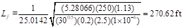
Find the well-fault distance using Eqs. (18) and (22):
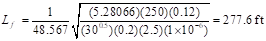
If the system were isotropic, the well-fault distance would be estimated with Eq. (23).
4.2. Synthetic example 2
Find the distance from the well to a constant-pressure linear boundary using the data given in Table 1 and the pressure derivative plot of Fig. 8.
Solution. The following data were taken from Fig. 8.
Reservoir permeability is found with Eq.(27), and the anisotropy angle factor is found using Eq.(19):

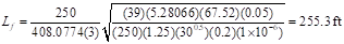
Find the distance from the well to the linear boundary using Eqs. (22), (25) and (26):
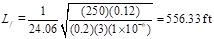
If the system were isotropic, the distance from the well to the linear boundary would be estimated to be the following by using Eq.(23):
4.3. Field example
[14] presented field data for a pressure test run in a well near a sealing fault in an anisotropic system. Pressure and pressure derivative versus time data are provided in Fig. 9. Finding the distance from well to the fault is required.
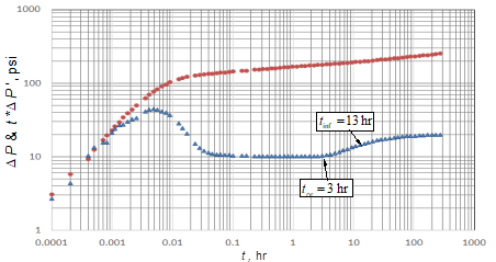
Solution. The following information was taken from Fig. 9.

Find the anisotropy angle factor using Eq.(19):

Find the well-fault distance using Eqs. (18) and (22):
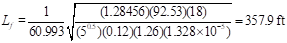
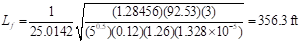
If the system were isotropic, the well-to-fault distance would be estimated using Eq.(23).
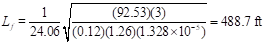
[14] estimated L f = 462.24 ft. The authors corrected the apparent distance estimated with Eq.(23) by using a reading from Fig. 9 by [23]. We found, however, that the correction factor was not estimated well. Then, we interpreted the test with a commercial software and found the well-to-fault distance to be 370 ft. This value was then used as our reference value for the estimation of the error.
5. Discussion of results
Table 2 provides the deviation error obtained for the working exercises. The proposed equations provided error values lower than 4%. The higher error was obtained from Eq.(25), which uses any point on the negative unit slope line.
Table 2 Deviation errors from the working examples
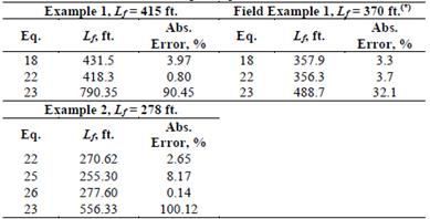
(*) Commercial interpretation software
Source: Authors
It is important to remark that the estimations provide deviation errors higher than 30% for the actual field case and even higher than 90% for the synthetic examples when the system is dealt as an isotropic case.
6. Conclusions
Practical and accurate expressions using the unique features of the pressure derivative plot were developed to determine the distance from a well to a linear boundary (constant-pressure or sealing fault) in areal anisotropic reservoirs. The expressions-successfully tested with two simulated examples and one field case example-simultaneously involve the anisotropy angle and the anisotropic index. Most of the developed expressions provided errors lower than 4%, except for one expression that uses an arbitrary point on the negative-unit-slope line.
The pressure derivative as a function of ( FC t D /(I A 0.5 L f 0.5) always displays the same behavior for wells near a linear boundary. The anisotropy angle factor, ( FC , has different estimations if the angle is less or higher than 45(. The relationship ( FC t D /(I A 0.5 L f 0.5) forms the basis of the methodology developed in this work.
Determination of the well-discontinuity distance using the isotropic formulae can provide errors even higher than 100%. For the real example, the error was 32%.