


 English (pdf)
 Article in xml format
 Article references
 Send this article by e-mail
 Cited by SciELO
  Cited by Google
  Similars in
SciELO
Similars in
SciELO  Similars in Google
 Permalink
1. Introduction
From the beginning of the study of the probability of repairable component failures, until now, operational availability is considered as the capacity of a component to fulfill its function when required [1-4]. This indicator originated because operational systems cannot guarantee 100% of the continuous flow of their operation, due to interruptions that occur as a result of the occurrence of unforeseen failures or the execution of preventive maintenance activities; therefore, they cannot fulfill their function during all the required time.
For this reason, availability is one of the most important indicators for decision making within operational and maintenance management [3,5], frequently used in the planning of the operation of productive and services systems.
Depending of system operational capacity, a small variation in availability represent very important variations in the operational consequences. For example, commonly in production systems, a small decrease in availability represents a considerable reduction in production [6]. So, the calculation of availability must have a high degree of accuracy.
The problem is that the calculation of the availability of a single component that is done by dividing the real operating time for the desired operating time [1,4] is consistent; but for series and parallel systems, the current calculation method [7-9] is analogous to that of reliability [10]; even though the availability and reliability are totally different.
Reliability is a purely stochastic process, which indicates the probability of satisfactory operation [3,11], whose value starts in one after the start-up or immediately after the repair and tends to zero when time tends to infinity; while, at the time the fault occurs and while it lasts, it takes the value of zero.
On the other hand, the operational availability is eminently deterministic, whose value in conjunction with other indicators measures the performance of the component during the analyzed time period; therefore, it expresses the result of events that occurred, and that for no reason is probabilistic. For this reason, the current equations for the calculation of the availability on series and parallel systems are questionable; however, these equations are widely used both in scientific research [12-14] and in the production of books [15,16].
The objective of this research is to evaluate these equations by analyzing the quantity of products that the system stops manufacturing due to the unavailability of each of its components, in order to know its level of precision and its calculation error. In order to do so, three operational models have been designed with two components each of equal operational capacity; set up in series, active parallel and passive parallel, respectively.
The results are obtained through the iteration of 5000 samples of size 250 with the Monte Carlo method, where a range of values of the down times of each component are entered randomly, in the current equations of the availability on series and parallel systems, to later evaluate its effectiveness, comparing these results with the t statistic.
2. Methodology
2.1. Foundations
With the purpose of using standard nomenclature and to have a better understanding of the relationship between the times used for the calculation of availability, an adaptation of the scheme of the "states of an item" of the EN 13306:2010 standard was made [17] in terms of the relative times to availability, obtaining the simplified scheme of Fig. 1.
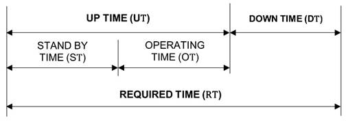
For the calculation of the individual availability of each component, eq. (1) corresponding to technical indicator T2 provided in standard EN 15341:2007 [18]. In terms of Fig. 1, this indicator is expressed as follows:
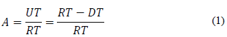
Where A is availability, UT is up time obtained during the required time, DT is down time obtained during the required time and RT is the required time.
The amount of production reached on production system depends on the intrinsic operating capacity of a certain production process under certain operating conditions and the total effective time in which that process works without failure. This is reflected with the following equation:
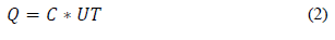
Where Q is the production reached and C is the operational capacity expressed in items produced by time unit.
On the other hand, the production not manufactured as a consequence of the down time ( ) is calculated with:
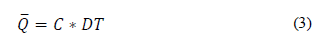
To express in terms of availability, eq. (1) was replaced in eq. (3), having as a result:

Note that the production reached plus the non-manufactured production as a consequence of the down time is the installed capacity (Q0).
2.2. Models of the systems
The model of series system was delimited with two components as illustrated in Fig. 2. This model is characterized in that any functional failure of one of its components causes the failure of the entire system [5,15]. Therefore, if component 1 is in a fault state, the system will not be able to operate, remaining in a down state, while component 2 remains in the stand by state. Analogously, if component 2 is in a fault state, the system will not be able to operate either, at which time component 1 will be in the stand by state.
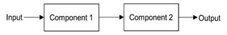
It should be noted that the component that is in the stand by state cannot fail because it is not operating; therefore, the total sum of the down times of each component, in no case can be greater than the required time, otherwise the equation (1) and those that are deducted from it, would give negative values, which is unreal.
In the model of the active parallel system indicated in Fig. 3, the two components operate simultaneously and with the same operating capacity, although in reality their capacities may be different. This model is characterized in that the functional failure of one of its components causes the decrease in the capacity of the system by half; therefore, the parallel system is in a down state only if the two components fail at the same time [5,15].
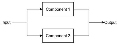
The model of passive parallel system was also represented with the two components of Fig. 3. This model is characterized by when component 1 fails, component 2 comes into operation, which is the one configured in passive parallel; Thus; as long as the two components do not fail at the same time, the system will continue to operate [15]. In this model the two components also have the same operational capacity.
2.3. Deterministic model
The deterministic model for the simulation using the Monte Carlo method was based on the current equations for calculating the availability of series and parallel systems, in order to determine the non-manufactured production as a consequence of the down time (eq. 4); and with the real reached production calculated with eq. (3). For which, the current equation for calculation of the availability on series systems is the following [8]:
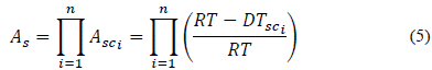
Where As is the availability on series system, Acsi is the availability of i th series component, DTsci is the down time of 𝑖th series component and n is the total number of series components.
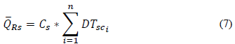
The non-manufactured production as down time consequence of series systems was obtained by replacing the eq. (5) in eq. (4):
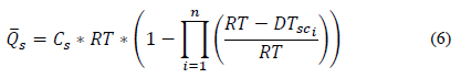
Where  is the non-manufactured production as down time consequence on series system and C
s
𝐶 𝑠 is the operational capacity on series system.
is the non-manufactured production as down time consequence on series system and C
s
𝐶 𝑠 is the operational capacity on series system.
The real reached production of the series system of Fig. 2 was determined by eq. (3), and considering that, from the point of view of availability, a serial system behaves as if it were a single operating unit (equipment, device); in such virtue, the down time of this operative unit is equal to the sum of the individual down times of its components.
Where  is the real non-manufactured production as a result of the down time on series system and
  is the total down time on serial system achieved during the required time.
The current equation for calculating the availability on parallel systems, both active and passive, is following [8]:
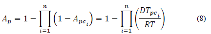
Where A p is the availability of active or passive parallel system, A pci is the availability of 𝑖th active or passive parallel component, DT pci is the down time of i th active or passive parallel component and n is the total number of parallel components.
The non-manufactured production as a consequence of the down time on active or passive parallel systems was obtained by replacing eq. (8) in eq. (4):
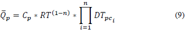
Where  is the non-manufactured production as result of down time on active or passive parallel system, C
p
is the operational capacity on active or passive parallel system and DT
pci
𝐷𝑇 𝑝𝑐 𝑖 is the down time of i th component on active or passive parallel system.
is the non-manufactured production as result of down time on active or passive parallel system, C
p
is the operational capacity on active or passive parallel system and DT
pci
𝐷𝑇 𝑝𝑐 𝑖 is the down time of i th component on active or passive parallel system.
The real production reached on active parallel system was determined considering that, in this case, each of the components delivers its production quota individually, in such a way that the production reached by the system is equal to the sum of productions reached for each of its components. Similarly, non-manufactured production as a result of the down time on active parallel system is equal to the sum of the non-manufactured production of each of its components.
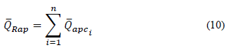
Where  is the real non-manufactured production as a result of the down time on active parallel system and
  is the real non-manufactured production as a result of the down time of 𝑖th active parallel component.
The real non-manufactured production as a result of the down time on active parallel system may be expressed in terms of the down time by replacing the eq (2) in eq. (10):
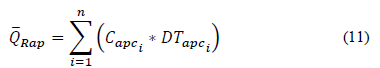
Where C apci is the operational capacity of i th active parallel component.
In order to determine the real reached production on passive parallel system, it was considered that, in these systems, one of the components operates actively, while the other one is in stand by state, entering into operation only if the active component suffers an operational failure, preventing production from falling. Consequently, non-manufactured products will be generated only if the two components are simultaneously in a down state; Thus:
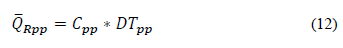
Where  is the real non-manufactured production as a result of down time on passive parallel system, C
pp
is the operational capacity on passive parallel system and DT
pp
is the simultaneous down time of the two components.
is the real non-manufactured production as a result of down time on passive parallel system, C
pp
is the operational capacity on passive parallel system and DT
pp
is the simultaneous down time of the two components.
2.4. Monte Carlo method
In all the deterministic model equations (eqs. 6, 7, 9, 11 and 12), 40 hours were pondered for the required time, since this is the total number of hours that is completed from Monday to Friday with a normal working time of 8 hours daily.
In accordance with the characteristics of series systems exposed in the section "Models of the systems ", it was established that in the stochastic process 20 hours were generated as the maximum random value for the down time of components 1 and 2, so as not to create the possibility that in some iteration the total sum of the down times of eq. (7) exceed required time equal to 40 hours.
Extending this condition for all deterministic models, it was established that the random entries of down times of components 1 and 2 must be in range of 0 to 20 hours.
To facilitate the processing of the data, the operational capacity of each of the three modeled systems was pondered at 100 units per hour.
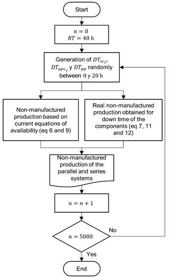
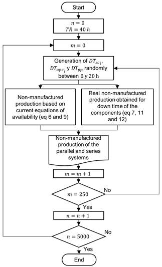
The simulations were elaborated using algorithms of Figs. 4 and 5, where the stochastic process was developed with the random generation of the down times on series and parallel systems (DT sci, DT apci, and DT pp ), while the deterministic model was satisfied with the calculations of the non-manufactured production with eqs. (6), (7), (9), (11) and (12).
To guarantee that the random generation of stochastic process down times may covers the range from 0 to 20 hours, five thousand iterations were performed; while for the comparison of the results of the equations to be analyzed and because many data may be generated with the Monte Carlo method, the central limit theorem with 5000 samples of size 250 (Fig. 5) was used to obtain a good approximation [19].
The statistical software R, version 3.5.1 was used to obtain the data and for its subsequent analysis.
3. Results and analysis
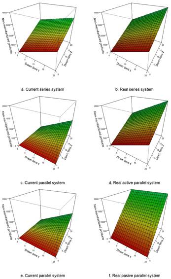
Before the statistical treatment of the data, it is important to make a comparison of the current and real equations of the series and parallel systems, this is done through the three-dimensional graphs of Fig. 6, where the dependent variable is the non-manufactured products which is represented on the z axis; while the independent variables are defined by the down times 1 and 2 corresponding to the x and y axes respectively.
In Fig. 6 it may be observed that in all cases there is a positive tendency that starts from the origin; however, when the down time reaches 20 hours, the non-manufactured production differs between current and real methods. In order to have a better appreciation of these differences, the non-manufactured production is tabulated in Tables 1, 2 and 3 when the down times are extreme (0 and 20 hours).
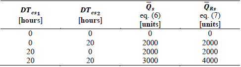
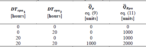
As indicated in Table 1, on series system, half the required time (20 hours) the component 1 fails and the other half (20 hours) fails the component 2, giving a total of 40 hours, but the system did not operate during this time. Therefore, the non-manufactured production is equal to the nominal production (4000 units), as indicated in eq. (7). However, with the current equation, 3000 non- manufactured units were obtained, which suggests that, although the system did not operate at any time, 1000 units were manufactured. Result that is impossible to obtain in reality.
Source: The authors.
Figure 5 Algorithm for simulation through the Monte Carlo method for the analysis using the central limit theorem.
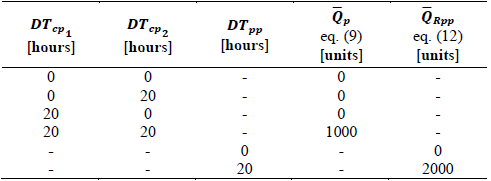
For the active parallel system to have a capacity of 100 units per hour (which is the initial condition of the simulation), each component has to operate with a capacity of 50 units per hour. If in the half of the required time, the component 1 fails and component 2 fails in the other half of required time, the system operates only whit one component at a time, which means that its capacity is reduced by half, generating a non-manufactured production of 2000 units, as indicated in the last row of Table 2 with eq. (11)
While with the eq. (9), the non-manufactured production is less than the real one; but the most remarkable thing occurs when only one of the two active parallel component has a down time equal zero, the non-manufactured production is not generated, reaching the nominal production; although, only one component is operated; thus, eq (9) does not fit as expected.
Source: The authors.
Figure 6 Graphical comparison of current and real functions of series and parallel systems
Concerning passive parallel systems, their components operate one at a time. In no case operate both at the same time, since the component 2 is a backup, coming into operation, only when the first has failed. These systems are the most reliable, generating non-manufactured production when the main component fails at the same time that the backup component is inoperative (eq. (12) of Table 3).
On the other hand, eq. (9) admits down times without any condition, enabling the generation of non-manufactured production when the two components fail at different time points. So, the eq. (9) neither fits as expected in these systems.
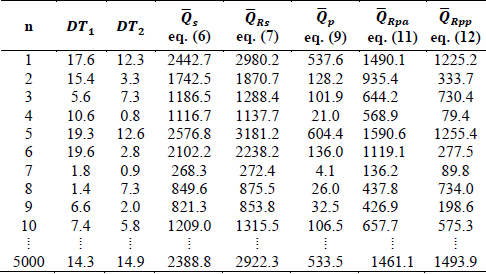
So far, significant differences may be observed between the real data and those obtained with the current equations; but to make a more effective comparison it is necessary to analyze a lot of cases. For this purpose, the simulation of the algorithm of Fig. 4 is used; in which, the results of the first ten and the last iteration are indicated in Table 4, where DT1 and DT2 are the down times of components 1 and 2 of the systems models of Fig. 2 and 3 respectively, those were obtained randomly in order to be replaced in eq. (6), (7), (9), (11) and (12) in each of the iterations.
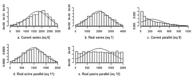
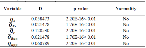
The relative frequency histograms of the results obtained in the 5000 iterations are indicated in Fig. 7, where it is observed that the data does not seem to have a normal distribution, for this reason an analytical normality test is carried out using the Kolmogorov Smirnov method with the modification of Lilliefors, obtaining as a result that none of the variables evaluated are normally distributed, with a confidence of 99%, since in each case the p-value of the test statistic is less than 0.01 (Table 5).
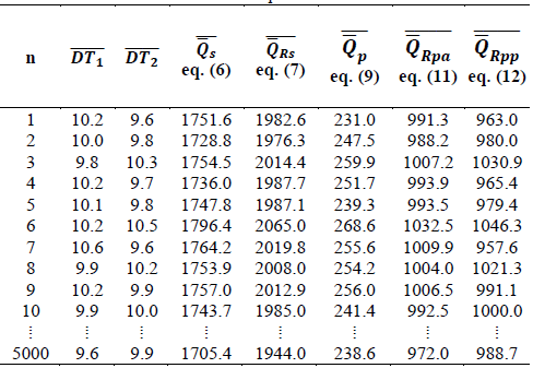
Due to the large amount of data that may be obtained through the simulations, it is decided to apply the central limit theorem with 5000 samples of size 250, which is sufficient for the sample means to be distributed normally. The results of the first 10 sample means and the last one is indicated in Table 6 and their respective relative frequency histograms are shown in Fig. 8, which seem to be normally distributed.
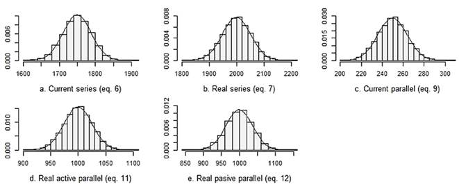
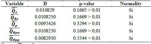
Indeed, the analysis of normality by the Kolmogorov Smirnov method with the modification of Lilliefors indicated in Table 7, shows that the sample means of the variables evaluated from the non-manufactured production on series and parallel systems are normally distributed, with a 99% confidence, since in each case the p-value of the statistic test is greater than 0.01.
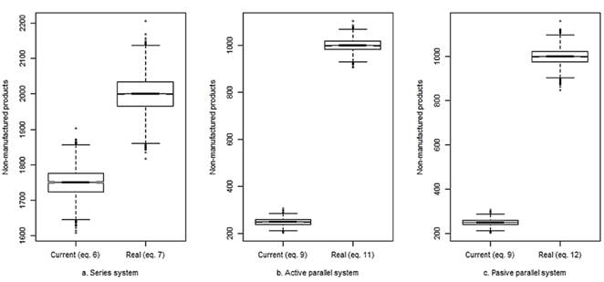
In the statistical comparison by means of the box diagrams of Fig. 9. it can be seen that there is a clear difference between the results of the non-manufactured products calculated with the current equations and the real ones on series and parallel systems. This observation must be confirmed by using analytical statistical methods.
Source: The authors.
Figure 9 Box diagrams of the sample means of the results of the non-manufactured products calculated with the current equations and the real ones.
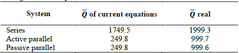
Given that, the sample means of the variables have a normal distribution, it proceeds to evaluate the efficacy of the current equations by means of the parametric statistic t; where the H0 corresponds to the equality of the sample means, which indicates that the current equations are effective. The averages of the sample means are indicated in Table 8, while the results of this test are shown in Table 9.
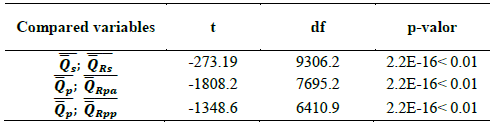
Since the p-value obtained with the t statistic is less than 0.01 for each of the systems (Table 9), the H0 is rejected, therefore, there is sufficient evidence to demonstrate that the two samples have different measures with the 99% confidence in each case, which means that the current equations for the calculation of the availability on series and parallel systems, give different results in comparison with the real ones.
4. Conclusions
The production losses are proportional to the down time of each system component, for this reason this calculation may be used to deduce an equation that relates the non-manufactured production with the availability of each component of series and parallel system.
The non-manufactured products resulting from the simulations using the Monte Carlo method are not normally distributed in the three systems analyzed; however, the sample means when applying the central limit theorem are distributed normally. They allow to evaluate the data by parametric methods.
The t statistic test that allows to compare of sample means distributions, shows that the current equations are ineffective with a confidence of 99%.

