


 Inglés (pdf)
 Articulo en XML
 Referencias del artículo
 Enviar articulo por email
 Citado por SciELO
  Citado por Google
  Similares en
SciELO
Similares en
SciELO  Similares en Google
 Permalink
1. Introduction
Meat and processed meat products are highly perishable foods that are characterized by a short shelf life, which is why it is important to properly handle post-production preservation processes. Temperature is the most important and influential factor in the quality and safety of these foods because if the storage and transportation conditions are inadequate with respect to the temperature, the shelf life will be considerably reduced [1]. Therefore, it would negatively affect the sales forecast of the product. In addition, temperature excesses increase the growth rates and survival of pathogenic microorganisms as well as increase the potential for toxin production [2]. On the other hand, the manufacturing processes involve manipulations that can lead to microbial contamination at refrigeration temperatures considered to be extreme. Thus, storage temperature is one of the most important factors affecting food safety and quality because it directly influences microbial growth and consequently the associated risk of foodborne diseases (FBDs) [3,4]. In addition, inadequate temperature is second on the list of factors that cause FBDs, surpassed only by the initial microbial population present in the food [5].
Consequently, meat and meat products have to be processed, stored and transported under cold conditions within a temperature range of 2°C to 7°C depending on the type of product; each degree outside the given temperature range leads to a reduction in the shelf life [1], which also leads to considerable economic loss. Different authors have reported that the main problems related to incorrect temperature conditions occur at the points of the transfer of products from one place to another [6,7].
In this way, each product has a shelf life defined by an expiration date, which is established when the product is packaged at the end of the processing line. According to Colombian Resolution 2652 of 2004, the expiration date is the date set by the manufacturer, which ends the period after which the product, stored under the indicated conditions, will probably not have the quality attributes normally expected by consumers. After this date, the food will not be considered marketable. This date is linked, in addition to other factors, to the amount of microorganisms that can develop in the product over a certain period of time. The shelf life of the meat products depend, among others, on the maintenance and conservation of the cold chain, referring to the continuous process of the production, packaging and distribution of a temperature-sensitive product [8]. Thus, the shelf life defined by the producer cannot reflect the actual time of deterioration because it is deliberately estimated, in most cases, by not taking temperature changes during storage into account [9]. Therefore, one of the best methods to define the actual date when the product should be withdrawn from the market is to predict its actual shelf life [9].
The remaining shelf life of the product at each step in the supply chain can be estimated using methods such as traditional microbiological analyses. Although it is still difficult for companies to draw conclusions about the shelf life based solely on temperature data, the determination of the shelf life optimizes the product’s management and storage in order to minimize the economic losses [10].
Therefore, more and more food producers are looking for intelligent systems that are able to predict the shelf life of a product after its transformation and also allow a calculation of the remaining life at each step of the cold chain. Thus, an alternative to costly research and time spent on the microbiological analyses of this type of product is microbiological prediction using mathematical models for predicting the growth, mortality, and survival of microorganisms [11].
Currently there are different models for predicting the shelf life of microorganisms; however, these methods have restrictions for their application in the meat industry due to factors that are not included in the direct operation of a meat business, which are associated with indirect costs such as the history of the growth of microorganisms, characterization of the growth of microorganisms [12], kinetic parameters in equations and constant temperature monitoring during growth [13,14].
1.1. Predictive models of microorganism growth
One area of food microbiology is predictive microbiology. It was defined as a quantitative science that allows users to objectively evaluate the effects of processing, distribution and storage operations on microbiological safety and food quality [15]. The goal of predictive microbiology is to develop mathematical equations that describe the behavior of microorganisms under the following different environmental factors: physical, chemical, and competitive [16-18]. The most important objective of predictive microbiology is to understand and predict the behavior of microbial ecosystems, which are very complex subjects to study because they show variable patterns in both the temporal and spatial domains that are still difficult to explain [19].
In science, mathematical models are essential in the construction of prediction tools, but in this study, traditional models of predictive microbiology do not work for the construction of the model because to build a predictive model with growth dynamics, the experimental data must be generated at constant temperature, and then a mathematical model (primary model) is developed to describe the relationship between the microbial population in food and storage time. Subsequently the dependence of the parameters used in the model on temperature is evaluated, which is considered a secondary model [20,21].
1.2. Quadratic model for the construction of the predictive model
Microbial growth is often sigmoidal and can be described by the S curve or logistic curve [9]. This is a model commonly used to study and modify future changes [22]; however, inadequate application of the S curve leads to very inaccurate results [23]. Thus, a straight line can be fitted to an S-curve if the beginning and end of the periods that compose it is ignored, but to establish the real growth of a population, for example, another type of information is required [23]. Therefore, it is important to know when this model can be used taking into account how to define the system, how to identify relevant growth variables for long-term forecasting, how to improve model and data consistency, and how to interpret the curve obtained [22]. In general, one should have good reason to believe that a fit of the S curve is appropriate [23]. When the population growth data are adjusted to the S curve, the model function tends to represent the trend curve of the data when these three parameters are known: (1) saturation, (2) growth time, and (3) mid-point. The first refers to the growth limit, the second refers to the time it takes to grow from 10% to 90%, and the third refers to the inflection point of the curve [22].
Thus, to apply the S curve, one must know the adaptation phase of the microorganisms, but for the construction of the model in this particular case, the growth history of the microorganism to be studied is unknown, and the requirement of multiple variables makes it very complex to manipulate and/or adapt the S curve. However, assuming that microorganisms have this type of growth behavior, the authors propose approximating this S curve by sections, where each section is modeled as a multivariate quadratic equation.
The most common measurement to determine the quality of prediction is the coefficient of determination R2 used in linear regression models [24]. In the linear context, it is a very intuitive measurement because values between 0 and 1 provide a quick interpretation of how much of the variance of the data is explained by the fit [25]. However, the statistic R2 is an inadequate measurement to determine the quality of fit of non-linear regression models [25]. For this reason, the mean absolute percentage error (MAPE) has been used to find the error of the model; that is, it interprets errors in a percentage form, facilitating their comparison because it expresses the accuracy of the model as a percentage of the error [26].
1.3 Normativity of meat products in Colombia
In Colombia, NTC 1325 of 2008 establishes the requirements that non-canned processed meat products must meet. This includes the microbiological requirements for this type of food. The most important requirement for this case study is the maximum permissible index of mesophilic aerobic microorganisms, which identifies the acceptable level of quality for cooked processed meat products of 5 log CFU/g.
2 Methodology
During this research, a cooked processed meat product was used, which is defined by Colombian Technical Standard 1325 of 2008 as part of the carcass or muscular portions of cured food-production animals that preserve their anatomical integrity and have undergone processes of being precooked or cooked or smoked or not smoked, including the following: cutlet, rib, tongue, loin, shank, processed legs, smoked turkey, and smoked chicken, among others. In this study, chilled processed cooked chorizo was used.
The steps to develop the predictive growth model for aerobic mesophilic microorganisms in the storage of finished products were established with the following criteria: (A) non-constant storage temperature and lack of knowledge of the adaptation phase or lag phase of mesophilic microorganisms, and (B) the model is developed for a Z population of indicator microorganisms and not for a species in general.
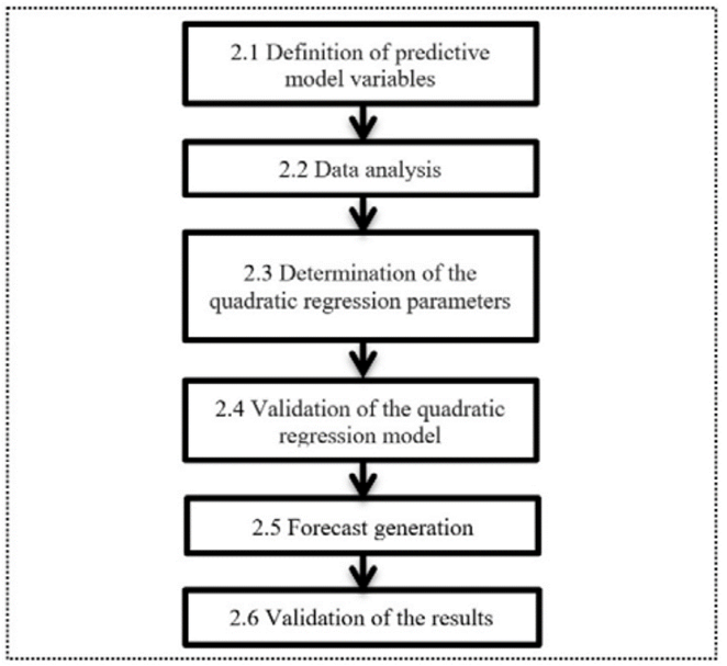
In the block diagram (Fig. 1), the main activities to construct the model are stated
2.1 Definition of predictive model variables
To define the variables of the model, the following concepts are defined:
Batch: independent production units with common characteristics. It consists of an amount of several packages of the same product.
Sample: a representative part of the batch that is used to carry out the microbiological analyses. A sample consists of a set of observations. The number of observations that compose the sample is called the sample size.
Study time (st): total time of the duration of the study equal to the shelf life of the product.
Variables in the predictive model include the following: (1) the dependent variable seeks to predict the population of aerobic mesophilic microorganisms (number of microorganisms) in different batches of the product from a sample taken from each batch, and (2) the following are the independent variables (or explanatory variables for the number of microorganisms) in this model:
Time: storage time of the finished product after leaving production. It is expressed in weeks, from week 0 to week "st", which correspond to the weeks of product shelf life.
Storage temperature: post-production temperature of the finished product, expressed in degrees centigrade (°C), which is measured weekly from week 0. Observations were taken in the refrigeration rooms where the finished and packaged product is stored.
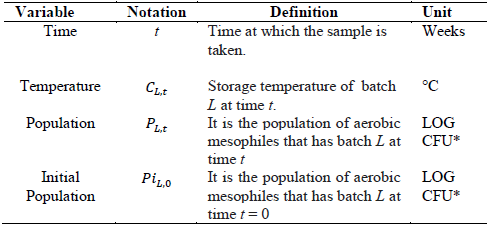
Initial population: population of aerobic mesophilic microorganisms of the finished product obtained at the time of production, (week 0). It is expressed in log CFU (logarithm of colony forming units). Table 1 shows the notation of each of the model variables.
2.2 Data analysis
To define the sample size (n) required for the construction of the model, one of the two methods could be used:
Heuristic rule: proposes that for multiple regressions, 20 observations for each of the independent variables that the regression model includes must be chosen. That is, the sample size is n=20*m, where m is the number of independent variables [27].
Green rule (1991): proposes a formula for determining the size of a sample for a regression model, which is described as n>50+8m, where m is the number of independent variables [28].
The two formulas above indicate the minimum number of observations required to construct a regression model. However, the formula that achieves the highest number of observations should be chosen because the out-of-sample forecast will be used [29]. This method is preferred because it divides the total observations into two sets: one to determine the parameters of the predictive model and the other in order to validate the accuracy of that model [30]. For the study model with three independent variables, it was decided to use the rule proposed by Green [28] because it requires a greater number of observations. This allows a sufficient amount of observations in each of the two sets.
Table 2 shows the observations taken for batch L.
Table 2 Sample results format.
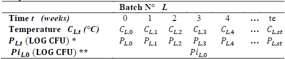
*P L.t (LOG CFU) = Population ** Pi L.0 (LOG CFU)= Initial population
Source: The Authors.
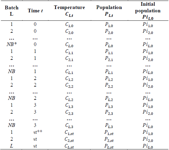
The observations obtained from each of the batches are then organized as shown in Table 3.
The total observations obtained in Table 3 are divided into two sets. The first is called a fit set, which corresponds to 80% of the total observations (nA observations) and must be used to construct the model (determine the values of its parameters). The second group is the test set, which corresponds to 20% of the observations (nP observations) and must be used to perform the validation of the model.
2.3 Determination of the quadratic regression parameters
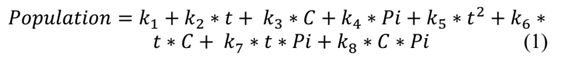
Minitab 17® software is used to determine the quadratic equation that best describes the observations of the fit set. Minitab 17® uses the least squares procedure to determine the values of the model parameters that minimize the sum of the squares of the differences between the observed values and those predicted by the fitted model, which are the residuals. Eq. (1) represents the quadratic model:
Finally, the MAPE is calculated, and eq. (2) describes the MAPE of the fit set:

Where 𝑦𝑖 is the real value,
 is the predicted value, and 𝑛𝐴 is the number of observations of the fit set.
2.4 Validation of the quadratic regression model
Validation is an essential step of the modeling process. Models cannot be applied without a pre-validation process. This typically consists of confirming predictions experimentally using any quantitative method [31].
To prove that the constructed model has predictive ability, the test set is used. To do this, the variables 𝑡, 𝐶, and 𝑃𝑖 are replaced in eq. (1), and the predicted results are compared with the actual values. Finally, the MAPE of the test set is found with eq. (3):

Where 𝑦𝑖 is the real value,
 is the predicted value and 𝑛P is the number of observations in the test set.
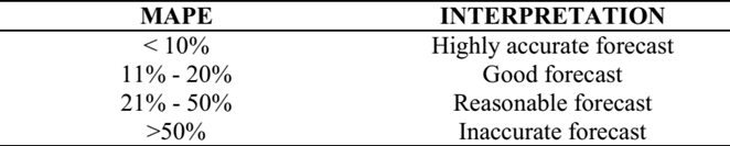
According to the result of the error, the model is accepted or rejected. For this, Lewis [32] developed a scale to assess the accuracy of the forecast using the MAPE indicator, which is presented in Table 4.
2.5 Forecast generation
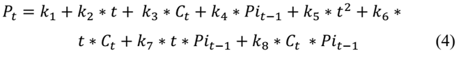
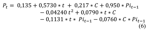
This step sought to identify the week in which the product exceeds the specified limit of aerobic mesophilic microorganisms defined by NTC 1325 of 2008. Eq. (4), which is a recursive equation to calculate the level of aerobic mesophilic microorganisms at the beginning of week t (𝑃𝑡), is based on the level of aerobic mesophilic microorganisms at the beginning of week t-1 (Pi t-1 = P t-1 ) and the temperature at the beginning of period t (𝐶𝑡). In this sense, P it-1 represents the population of mesophiles influenced by all temperatures prior to period t.
2.6 Validation of the results
In predictive microbiology, experimental analysis of the growth of microorganisms in food is the basis for validation of the results; experimental growth data are compared with model predictions [33]. To determine the efficiency of the predictive model, it is important to specify when predictions of the withdrawal dates of product batches are considered favorable cases and when they are considered unfavorable cases.
There are 3 types of favorable cases:
a. Type 1: Those cases in which the predicted data and actual data indicate the withdrawal of product from the distribution system in the same week it is stored based on the limit of aerobic mesophilic microorganisms established by NTC 1325 of 2008.
b. Type 2: Those cases in which the prediction indicates the withdrawal of the product from the distribution system one week before the actual date, based on the limit of aerobic mesophilic microorganisms established by NTC 1325 of 2008.
c. Type 3: Those cases in which the predicted data and actual data exceed week six complying with NTC 1325 of 2008 with less than 5 log CFU.
There are 2 types of unfavorable cases:
a. Those cases where the model predicts that the product should be withdrawn from the distribution system after the actual date, in relation to the limit of aerobic mesophilic microorganisms established by NTC 1325 of 2008. In other words, when comparing the predicted value and the actual value, the first indicates a withdrawal of the product one or more weeks after when it should actually be withdrawn according to actual results.
b. Those cases where the model predicts that the product should be withdrawn from the distribution system two or more weeks in advance of the actual value based on the limit of aerobic mesophilic microorganisms established by NTC 1325 of 2008.
3 Case study
The methodology proposed in section 2 was applied to a local meats products company, which was called EPPC for confidentiality. Packaged chilled processed cooked sausage was used as the product. Each package weighed 500 grams and contained 8 units of product. This product, if kept refrigerated between 0°C and 4°C, is assigned a shelf life of six weeks from the date of manufacture. EPPC had sampled 60 batches of the product for the quality control stage.
Below are the steps of the proposed methodology applied to the case study.
3.1 Definition of predictive model variables
The time, temperature and initial number of aerobic mesophilic microorganisms were defined as independent variables, and the population was described as the number of aerobic mesophilic microorganisms in each time-temperature condition. The shelf life of the product was six weeks (study period).
3.2 Data analysis
Observations were taken week by week, in cold rooms where the product is stored. For each of the batches, observations were taken from week 0 to week 6. Therefore, each batch should have 7 observations, one for each week of storage. Each observation can consist of several product packages, from which a sample pool is created to perform the corresponding microbiological analysis.
Subsequently, the sample size is defined for the construction of the model using the Green method (section 2.2). In this study, it gives a result of at least 74 observations. If for each batch there are 7 observations, following the equation L=
 , this corresponds to a minimum of 11 batches.
In this study, information came from 60 batches (NL = 60), which resulted in a number (420 observations) greater than the minimum recommended, and thus, it was decided to include all batches in the case study analysis.
The 420 observations were divided into two groups. The fit set had nA = 336 observations, and the test set contained nP = 84 observations.
To enter the observations of the fit and test sets into the Minitab 17® software, the information for each set was organized independently according to Table 2.
3.3 Determination of the parameters of the quadratic equation
Using the observations from the fit set, the values of the parameters shown in Table 5 were obtained.
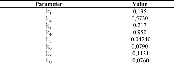
Therefore, eq. (5) represents the quadratic equation for the prediction of aerobic mesophiles with variable temperatures of the sausage product:
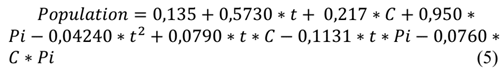
With the application of eq. (5) to the fit set, a MAPE of 6.7% was obtained, which, according to Lewis [32], is considered a very accurate fit of the prediction model, as the error was less than 10%.
3.4 Validation of the regression model
The validation of the multiple quadratic regression model was performed with the test set after replacing the variables t,C,Pi in eq. (5). A MAPE of 9% was obtained, indicating a very accurate forecast (Lewis [32]).
3.5 Forecast generation
The recursive eq. (6) was used to identify, in each batch, the week in which the product does not meet the requirement for the count of aerobic mesophilic microorganisms given by NTC 1325 of 2008, which stipulates that the maximum allowable index to identify a level of good quality is 5 log CFU.
3.6 Validation of results
The validation of the results was performed by comparing the resulting predicted values with eq. (6) against the actual values, and each batch was labeled as favorable or unfavorable.
In this way, 51 favorable cases and 9 unfavorable cases were obtained from the 60 batches evaluated, indicating an accuracy percentage of 91%. Thus, as stipulated in section 2.6, the 51 favorable cases are divided as follows: 27 type 1 cases, 3 type 2 cases and 21 type 3 cases.
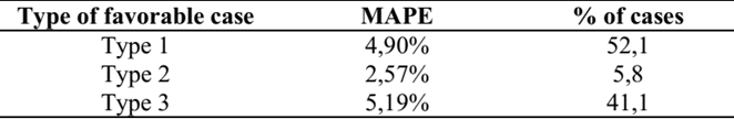
3.7 Supplementary analysis
Finally, the MAPE was found in each of the favorable types of cases presented. Based on the favorable cases obtained from the 60 batches evaluated, the percentages of types 1, 2 and 3 favorable cases were also found. The results obtained are listed in Table 6.
4. Conclusions and future work
The model proposed in this research has the ability to predict the behavior of aerobic mesophilic microorganisms in meat products at storage temperature conditions fluctuating between 1°C and 7°C.
In this manner, the model constitutes an important contribution to the meat industry by allowing the withdrawal date of the shelf life to be known more accurately according to storage conditions associated with temperature. With this, companies can more efficiently manage their inventory levels by estimating a sufficient quantity of product not only based on customer demand but also on the expiration date.
As future work, it is recommended to carry out the prediction model of other indicator or pathogenic microorganisms for other industries based on the proposed methodology. In addition, it is recommended to extend the prediction model to the supply chain, taking into account other types of storage. As for example, transport storage from one city to another taking into account the temperature changes that products suffer along the supply chain.


