


 English (pdf)
 Article in xml format
 Article references
 Send this article by e-mail
 Cited by SciELO
  Cited by Google
  Similars in
SciELO
Similars in
SciELO  Similars in Google
 Permalink
1 Introduction
Solar photovoltaic (PV) penetration still keeps increasing thanks to the low technology costs and the favorable renewable energy policies. For example, in 2016 Solar Photovoltaic (PV) installed capacity grew by 50%, with half of such expansion in China [1]. PV generation accounts for up to 90% in the United States of America and for distributed energy sources with 2 MW or less of installed capacity [2]. According to the International Energy Agency [3], China and USA lead the annual installed capacity of solar generation with 34 and 14 GW. Besides, countries such as Japan, India, the United Kingdom, Germany, Korea, Australia, Philippines and Chile are over the mark of 700 MW of annual installed capacity [3].
For any amount of solar energy available, optimal exploitation of Distributed Energy Resources (DERs) in power distribution networks must always satisfy two conditions: a) physical laws that rule all electrical circuits; and b) power and service quality requirements. Namely, power quality and service problems might arise if high penetrations are not handled properly [4]. On the other hand, because distribution networks are operated with a radial topology, reversed flows might cause protection and regulation devices malfunctioning [5-7]. Additionally, distribution networks have the following characteristics: 1) The 3-phase set of voltage and currents are unbalanced, 2) The R/X ratio is high, 3) The load models depend on the connection and steady state voltage variations. A 3-phase Alternating Current Optimal Power Flow (3φ-ACOPF) can handle these characteristics and properly exploit DERs in a power distribution network. Objective functions for this optimization problem depend heavily on the network agent to be analyzed, but often are focused more on the distribution system operator, e.g., load curtailment minimization to safely operate the network and optimal reactive dispatch for losses minimization [8,9]. Also, it is common to see PV curtailment minimization [2,10] as an objective. Solution methods are mainly based on Interior Point Methods, however, as presented below, problem formulations vary widely.
1.1. Literature review
In general, the transmission Alternating Current Optimal Power Flow (ACOPF) is not appropriate to find the optimal DER schedules in a distribution network. However, some key ideas can be borrowed from advances in ACOPF. For example, in [11] a single phase ACOPF is solved as a sequence of Linear Programs which can be extended to solve the Unit Commitment problem [12]. A closer look reveals that this cartesian formulation allows the inclusion of constant current and constant impedance load models as linear constraints. This might lead to some computation performance and convergence improvements [13].
Interior Point (IP) algorithms can solve non-linear formulations of the 3φ-ACOPF efficiently, being the Current Injection Method (CIM) in cartesian coordinates the most common solution formulation. This is because, although polar and cartesian formulations lead to similar results and time performances [2,14,15], the cartesian formulations are the preferred way to solve large and complex 3φ-ACOPF because of their robustness [2].
However, recent advances on convex optimization have shown its importance to unbalanced power network analysis. Robbins et al. [16] present a Quadratic Programming formulation for the 3φ-ACOPF that also gives a lower bound for the problem. There, the authors claim that branch-flow Second Order Cone Programming (SOCP) approaches [17] are unable to cope with system unbalance. Moreover, Christakou et al. [18] show that branch-flow formulations also may introduce errors in branch currents for congested networks.
Ahmadi et al [19] present another alternative to SOCP formulations. They study how the linear approximation over a bounded region can be useful for the solution of three-phase power flow equations. Watson et al. [20] propose a non-iterative convex formulation to solve a 3φ-ACOPF, to analyze the effects of the neutral conductor and system storage in a distribution network. Additionally, Zamzam et al. [21] present a non-convex Quadratically Constraint Quadratic Programming formulation that also helps to find problematic constraints thanks to their Feasible Point Pursuit Successive Convex Approximation algorithm. In general, recent advances have presented Quadratic Programming as a promising alternative [22,23].
Convex alternatives to SOCP formulations are usually based on Semidefinite Programming (SDP). However, their use has been very limited, mainly because of two reasons: (1) SDP optimum computation is a resource intensive task; (2) SDP optimum depend heavily on the network itself. The time performance problem is solved by Li et al. [24] by using an SDP equivalent of the SOCP branch-flow formulation for the unbalanced problem. Another approach to solve the SDP limitations is based on finding a network partition that exploits chordal sparsity of the SDP formulation [25,26]. In particular, the network dependency is addressed in [25] by solving the 3φ-ACOPF as a sequence of SDP problems. From the former review, one can see that linear and convex approximations are important because they allow the inclusion of integer variables to 3φ-ACOPF [27] and it can be used to derive distribution network locational marginal prices [28].
1.2. Contributions
This paper presents an optimal DER scheduling algorithm for unbalanced distribution networks considering a full 3φ-ACOPF formulation which is solved as a sequence of convex Quadratically Constrained Quadratic Programs. This formulation is a novel solution that accounts explicitly for all relevant aspects of a power distribution network, including ZIP and delta loads. Moreover, the algorithm is able to find a primal feasible point for the non-linear formulation, making unnecessary approximations for the constant power component of a ZIP load model. Also, the presented algorithm is computationally more efficient than the IP method used as reference and it results in solutions with lower voltage unbalance.
1.3. Outline
This paper is organized as follows: Section 2 and 3 present the mathematical nomenclature and the distribution network models used. Section 4 describes the model approximations, while section 5 describes the optimization problem. Section 6 describes the 12 simulated cases. Section 7 presents the results and section 8 closes with some concluding remarks.
2. Nomenclature
The three-phase Alternating Current Optimal Power Flow (3φ-ACOPF) model presented below uses the following basic nomenclature: For an electric distribution network, let N={1,2,3…N} be the set of nodes and R={1,2,3…R} be the set of branches -each branch r Є R is defined by a pair of nodes n,m,. Є N Now, let g, D, and ф be the set of elements that inject power into the network, the set of loads and the set of phases, respectively. A subindex in any set indicates that a specific partition is being made, e.g., for a node n Є N and a generator g Є g, ,gn is the set of generators connected to node n, Ng is the set of nodes to which a generator g is connected, and фg is the set of phases that generator g has. Voltages are represented with the letter V, currents with I, apparent power with S (active power with P and reactive power with Q), impedance with Z and admittance with Y. A superscript ф is used to denote that the electrical variable is measured at phase ф. All electrical variables and parameters are presented as complex values when required, so for a complex number C, its complex conjugate is denoted by C*;Re{C}=Cr and lm{C}=Ci are their real and imaginary parts, respectively; and │C│ and <δc denote its magnitude and angle δc. To keep notation simple, all variables and constants are intended to be column vectors of complex numbers. Each component of the vector is the value of the variable in the corresponding time period, e.g. C=[C1,C2…Cτ]τ for a time window τ={1,2,…τ} and where Ct is the value variable  has at time t, and τ is the total number of time periods. With this in mind, all operations and equations are supposed to be time-component wise, e.g., for two complex vectors A and B, and τ = 2, mean and τ=2, A/B=C, mean A
1
/B
1
=C
1
and A
2
/B
2
=C
2.
has at time t, and τ is the total number of time periods. With this in mind, all operations and equations are supposed to be time-component wise, e.g., for two complex vectors A and B, and τ = 2, mean and τ=2, A/B=C, mean A
1
/B
1
=C
1
and A
2
/B
2
=C
2.
3. Models
Model equations are classified into three groups: Generation, demand and network. The equations are handled to the solver in cartesian form, similarly to the non-linear formulation in [11]; and without using discrete variables for the storage model, as in [29]. Equations below are used to declare the optimization problems in section 5.
3.1. Generation
There are two basic kinds of power generation in Active Distribution Networks (ADNs): from the bulk transmission system and from Distributed Energy Resources (DERs). Transmission system power injections are done at the network header node, while DER power injections can be done at any node n Є N of the network. Then, the injected apparent power from the transmission system at phase Ф is defined as:
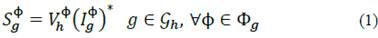
Where h is used to denote that the power from the transmission system is injected at the network header node, therefore, V ф h is the voltage at phase Ф of the network header node. Apparent power at system header is modeled just with eq. (1), in contrast, more details must be given to model DER power injections.
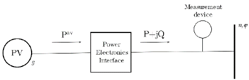
3.1.1. Photovoltaic system
Photovoltaic system active power injections are defined as the difference between the total available power and the curtailed power (see Fig. 1):
Where P av g . is the total available irradiance, p g is the total power being curtailed and P φ g, P φ g ≥0. Power curtailment is mainly used to avoid voltage limit violation. If there is no PV reactive power compensation, Q φ g =0. Otherwise, reactive power is limited by:

So, it always injects apparent power with at least a power factor equal to cosΘ max g
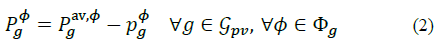
3.1.2. Storage system
In contrast to all other system elements, Electric Storage (ES) has two exclusive disjunctive states (charging and discharging), i.e., an ES can be charging or discharging, but not both. Therefore, its behavior can be modeled with auxiliary time-dependent Boolean (integer) variables. This drastically increase the problem complexity if it is done carelessly. Hence, since an efficient mixed-integer formulation of the storage system is beyond the scope of this paper, integer variables are avoided in the present formulation by choosing a proper objective function (see section 5.1.2) and by using the equations below (See Fig. 2).
Storage system active power injections are defined as:

Where  and
and  are the power being injected and withdrawn from the network; εin and εou are the efficiencies when injecting and withdrawing such power; and,
  . Besides, since for this study storage systems are not allowed to inject or withdraw reactive power,
  .
.
On the other hand, energy storage can connect two time periods. So, for any time period t, this property is defined by the following equation:
Where SOC is the state of charge of the storage system, and SOCфg,1= SOCфg,τ =SOCmin;Eg is the maximum storage energy, and Δt = 1 hour. Additionally, each storage system has the following constraints for all g Є gES and for all ф Є Фg

3.2. Demand
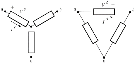
Power distribution network demand depends heavily on the type of connection and on the changes in power consumed due to changes in the steady state voltage applied. The two basic types of load connection are the wye and delta connection (see Fig. 3). The three basic types of load behavior considered here are the constant power, constant current and constant impedance behavior.
So, in first place, for any wye connected load, and NSY being the set of all nodes with constant (apparent) power injections; NSY being the set of all nodes with constant current injections; and NZY being the set of all nodes with constant impedance current injections; the demanded current equations are:
Source: The authors.
Figure 3 Wye (left) and delta (right) load connections. Branch voltage for the wye load is equal to the phase-to-neutral voltage, while for the delta load is equal to the phase-to-phase voltage.


Where DYn is the set of wye loads connected to node n, and  and
and  are the known wye load parameters of phase Φ that remain constant in spite of steady state voltage variations. From here, the total current injected at phase Φ of node n from a wye load d is defined as:

Secondly, for any delta connected load, and N S∆ being the set of all nodes with constant (apparent) power injections; N I∆ the set of all nodes with constant current injections; and N Z∆ the set of all nodes with constant impedance current injections; thus, the demanded current equations are:


Where D
∆n
is the set of delta loads connected to node n, Δ ={ф,ү} is a delta branch between phases ф and ү, and F= {(a, b), (b, c), (c, a)} (See Fig. 3);  and
and  are the known Δ branch load parameters that remain constant in spite of steady state voltage variations; and V
∆
n
is the applied voltage to the Δ branch, i.e.,
are the known Δ branch load parameters that remain constant in spite of steady state voltage variations; and V
∆
n
is the applied voltage to the Δ branch, i.e., 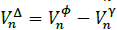 . Thus, the total current injected at phase φ of node n from a delta load d is defined as:
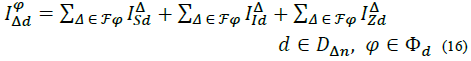
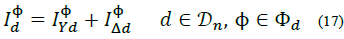
Where, F φ is the set of delta branches connected to phase φ, e.g., for φ =a = a, F φ = {(a, b), (a, c)}. Adding up everything, the total current demanded by a load d at phase ф of node n is:
3.3. Network
Two network components are treated: Lines and nodes. In contrast with previous elements, line equations involve variables from two nodes. Let us apply KCL to the line model depicted in Fig. 4:
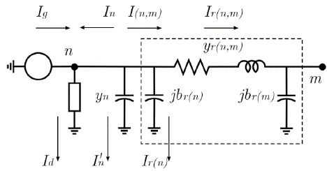


Where jbr(n)=yr(n) is the shunt susceptance of branch r at node n, yr(n,m) is the serial admittance of branch r, Ir(n) is the current flowing through yr(n) ,Ir(n,m) is the current flowing from node n to node m through yr(n,m), Vn is the voltage at node n and Vm is the voltage at node m -Note that yr(n,m) = yr(n,m) and yr(n,m)= yr(n,m). From eq. (20) and defining  and
and  , the current injected from the network at node 𝑛 is defined by:
Similar calculations can be done to deduce the three-phase line model, being the main difference the fact that each line shunt and series admittances are matrices for lines with more than one phase, hence, there are as much equations per branch as phases are on the branch:
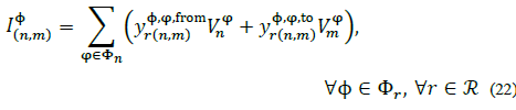
Where, φr is the set of all the phases connected to branch r ; and 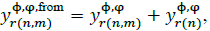 , with
 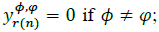 if Φ ≠ φ; and
 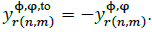 :
:
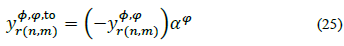
In order to include a voltage regulator in any branch, r eq. (22) must be modified in the following way (with tap on node n):
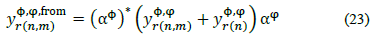
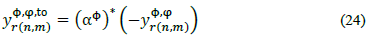
Where αф is the (constant) tap on phase ф. Furthermore, since 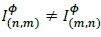 :
:
With the generation, demand and line current injections defined at node n, current balance must satisfy (see Fig. 2):
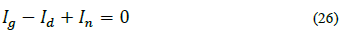
Where 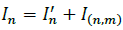 and.
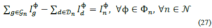
and.  Therefore, eq. (26) can be generalized as:
Where, 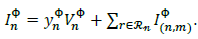 . Note that
  at nodes with neither generation nor demand.
Lower and upper voltage limits are implemented as follows:

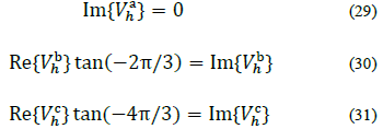
At the system header, voltage angles are fixed so they are fully balanced:
4. Model approximations
So far, the model presented has two sources of non-convexities: (1) The active/reactive power relationship with node voltages and currents (see eq. (1), (9), (13)); and, (2) The lower limit for the voltage magnitude (see eq. (28)). These set of equations will be treated as described below.
4.1. Power equations
If e denotes a circuit element (e.g., a generator or a constant apparent power component of a demand) for an operation point defined by the tuple 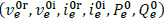 , eq. (1), (9), (13) are linearized using the First-Order Taylor approximation:
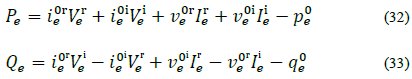
With, 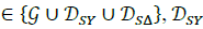 and D
s∆
being the sets of wye and delta constant power loads, and.
and D
s∆
being the sets of wye and delta constant power loads, and. 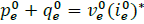 For example, from Fig. 3, one can see that for a wye or delta load, V
e
could be V
ф
or, V
∆
respectively.
For example, from Fig. 3, one can see that for a wye or delta load, V
e
could be V
ф
or, V
∆
respectively.
4.2. Voltage lower limit
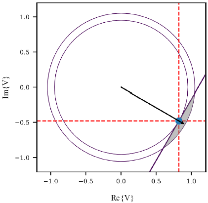
Preliminary testing with the linearized power equations resulted in good estimations for the active power injections and very poor approximations for the reactive power injections. Moreover, voltage angles were very close to those obtained by the non-linear model. This finding motivated the following approximation: Instead of the non-convex lower limit on eq. (28), the lower limit is modeled as a semiplane defined by a tangent line, so the upper and lower limits at phase Ф of node n are:
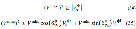
Where  is the phase Ф angle of the voltage at node n. In Fig. 5 there is an example of the new feasible region for a voltage that is on the fourth quadrant in the complex plane.
All other equations remain unaltered from the non-linear case, since they are linear or convex functions that can be handled by a Quadratically Constrained Programming (QCP) solver.
5. Problem definition
The Power Flow Equations (PFE) are defined by the following equations:
Thus, the power flow solution without DERs can be calculated by solving the PFE for a known voltage magnitude profile at system header and with. 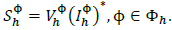
5.1. Non-linear formulation
Objectives of the Non-linear Programming (NLP) model are presented below, followed by the complete NLP formulation.
5.1.1. Active power losses
Total losses for each period of time in a three-phase power distribution system can be calculated as:

Assuming  :
:

Then, if  , and since
  and with Re
  for all connected phases, eq. (37) can be written as:
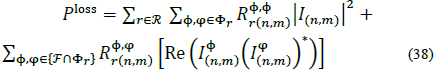
Note that eq. (36) gives the exact value for losses, while eq. (38) give a good estimate for distribution network losses. Therefore, the total active power losses can be defined as:
5.1.2. Storage arbitrage benefits
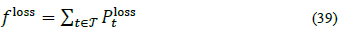
As reported in [29], by assuring that the round-trip efficiency of the storage system is less than one (i.e.,ε in ε ou <1 ), if power injections are meant to be maximized, and power withdrawals are meant to be minimized, one can model the storage device behavior without discrete variables if the following objective function is used:
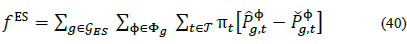
Assuming that energy is bought at the system header for a given price at each time t given by,  .
.
5.1.3 Problem formulation
The non-linear problem including PV reactive power compensation can be stated as follows:

5.2. Convex formulation
In addition to objectives described in eq. (39), (40), and to improve the quality and speed of the linearized power solution, the following objective function is included:
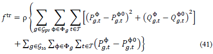
This trust-region objective assures that the next operation point does not fall too far from the current operation point depending on the value of p. This is useful near a NLP feasible operation point and, in most cases, it helps to find a better answer in terms of NLP primal feasibility.
Sequential Quadratic Constrained Quadratic Programing (S-QCP) formulation consists of 4 steps:
1) Initialize: All voltages initiate as a set of balanced phasors with a magnitude of 1 Vp.u.. Storage injections are set to 0, PV injections are equal to the given irradiance and for the trust-region objective function ρ = 0. Only initial values near the answer have significant impact on the method performance, otherwise, the problem final answer seems to be insensitive to initial values.
2) Solve: The QCP problem including PV reactive power compensation can be stated as follows:
 s.t. PFElin, eq. (3), (4-8), (34), (35)
Where PFElin are the power flow equations with the non-linear power injections replaced by their equivalent linearized power injections, i.e., with eq. (32)-(33) instead of eq. (1), (9), (13). In order to know when the trust-region objective must be included, the following index is calculated for all linearized power equations:
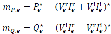
Where P*
e and Q
*
e
are the last optimal solution of the linearized model for element 𝑒. So, if max 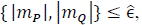 , for a given tolerance
  ,p=0; on the contrary p=0.
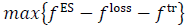
3) Stop: The algorithm will stop if max  given a tolerance level.Є It worth noticing that if all mismatch indices are zero, then, the S-QCP solution is a primal feasible point for the NLP problem. Additionally, NLP model simulation time is also used as stopping criteria. Also, every time the algorithm finishes this step, it is said that an outer iteration has been completed.
4) Update: If the tuple (V r e ,V i e ,P e ,Q e )* is the last solution of the QCP, then the next operation point is computed as follows:

After this, the rotating tangent lines are updated with the last solution for δ vn , and the algorithm returns to step 2.
6. Test cases
Models are tested for modified versions of the 13, 34 and 123 node IEEE test feeders [30]. Additionally, two scenarios were simulated for each circuit: a minimum scenario and a maximum scenario, having the latter twice the load and DER levels than the former; and both having 60% of PV penetration, i.e., total available irradiance accounts for 60% of the total active power imports at the header. Also, cases with and without PV reactive power compensation were simulated for each circuit and scenario, resulting in a total of twelve cases. Simulations were done for a 24 hour time lapse with a Δt equal to one hour. Solver tolerance parameters were set at 1 × 10− 6. The S-QCP tolerances where set to  = 1 × 10− 2 and Є= 1 × 10− 3.
Test feeders differ from the reference parameters only on tap setting values. On the other hand, load and available PV power are known. Load profiles were constructed from three basic types, while the PV profile is taken from available measures. All calculations are done under a per unit system, with a power base of 100 kVA and proper voltage bases.
All cases were implemented using GAMS 24.5.4, using IPOPT 3.12 solver (with MUMPS as linear solver) for the NLP model; and using CPLEX 12.6.2.0 solver for the S-QCP model. Simulations were done on a laptop computer with an Inter(R) Core(TM) i7-4700MQ processor (2.4GHz) with 6GB of RAM.
In addition to the decision variables and objective function optimal values, for each case is also computed the total active power consumption costs at the header  , and the average positive sequence node voltage, and negative and zero sequence Voltage Unbalance Factor (VUF) for each node.
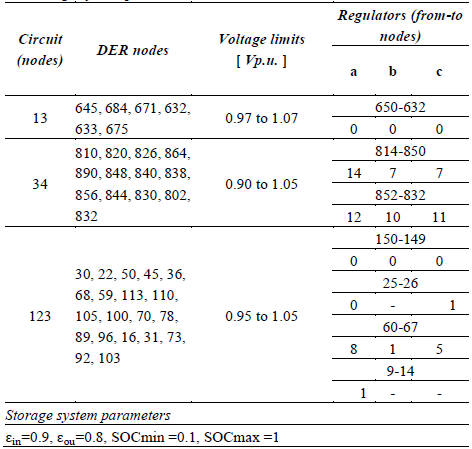
Table 1 describes the nodes where PV and ES systems are connected (DER nodes). Also, there are described the maximum and minimum voltage magnitude values for each circuit, along with the regulator tap settings and the ES parameters.
Table 1 Nodes with DER generation, voltage limits, regulator nodes and tap position, and storage system parameters for each simulated case.
Source: The authors.
7. Results
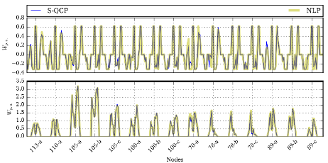
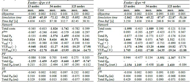
Table 2 shows the percentage differences between the NLP model and the S-QCP model for each of the twelve cases described in section 6. Note that the objective function from the S-QCP model differs by less than 0.25% with respect to its NLP counterpart in every tested case. Similarly, network losses and costs at the system header are very close between models. This is reaffirmed in Fig. 6, which depicts the active power injections for both models and all DERs of the IEEE 123 node test feeder. In general, both sets of active power injections are very alike.
Additionally, the S-QCP model finds a solution in less time than the NLP model (up to 87% faster, as seen in Table 2), and the maximum mismatch value is near 4.27 × 10− 4. Therefore, the computed solution can be considered as primal feasible for the NLP for a precision lower than 5 × 10− 4. It worth noticing that the mismatch is usually between 1 × 10− 5 and 1 × 10− 13, and such maximum values are uncommon.
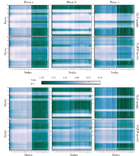
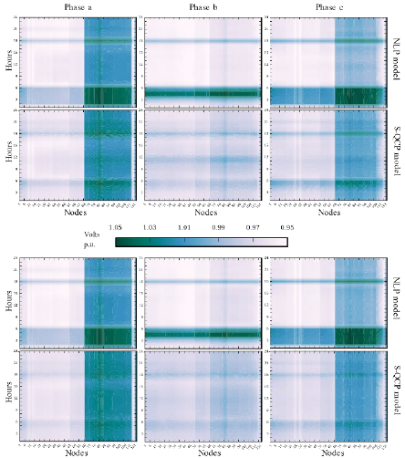
In Figs. 7 and 8 are depicted the voltage magnitude for all the twelves cases, for all the nodes and time periods of the 123 IEEE test feeder. There it is shown that the voltage differences are due to the approximation itself. For a given power injection, the relationship between node voltage and injected current is hyperbolic, thus, voltage profile is very sensitive to current injection variations, and therefore, voltage profile has sharp changes in the NLP model. In contrast, for the S-QCP model, for a given power injection the relationship between node voltage and injected current is linear, and so, the voltage profile is flatter because it is less sensitive to current injections than the NLP model. The latter can be seen in Fig. 7 and 8 as a more uniform distribution of color in the results of the S-QCP. As can be seen in Table 2, these flatter voltage profile in the S-QCP model causes higher differences on PV active power injections for the case without PV reactive compensation as well as higher differences in PV reactive compensation. In Fig. 9 are shown the voltage differences between the S-QCP model and the NLP model, for all the phases and PV penetration levels of the 123 node test feeder. There, a darker color indicates that the NLP model results in a lower voltage, while a lighter color indicates that the NLP model has a higher voltage. Therefore, the darker zone around the 19:00 hours for phases a and b and the maximum PV penetration, it is indicating that the NLP model decides to drop the node voltage as much as possible in order to withstand the active power injection. Additionally, the lighter zone before the 6:00 hours for the phase b of the minimum penetration scenario, it is indicating that the NLP model decides to increase the node voltage as much as possible in order to withstand the active power withdraw.
Source: The authors.
Figure 7 123 node test feeder voltage magnitudes for the max. scenario, with PV reactive compensation (first two rows) and without PV reactive compensation (last two rows).
Source: The authors.
Figure 8 123 node test feeder voltage magnitudes for the min. scenario, with PV reactive compensation (first two rows) and without PV reactive compensation (last two rows).
Table 2 Sequential QCP model percentage differences with respect to NLP model for each case. Time reference correspond to the NLP model.
Source: The authors.
Source: The authors.
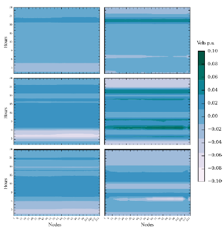
Figure 9 Voltage differences between S-QCP model and NLP model, for each phase (a -up, b -middle, c -down) and each scenario (minimum -left- and maximum -right- load and DER levels) of the 123 node test feeder with PV reactive compensation.
Also note that voltage differences of Fig. 9 are lacking vertical lighter or darker areas. This means that voltage differences between nodes for the NLP and the S-QCP models are very similar. Voltage differences are then more sensitive to changes between time periods, because of the differences between the active/reactive power needed to maintain the optimal voltage magnitude.
Despite of the differences listed above, resulting reactive power, voltage magnitude and voltage unbalance differences are not large enough to change the active power flows in the system. Tested cases suggest that those differences depend mainly on the system topology and the required operation parameters (e.g. PV curtailment and voltages limits). Also note that the S-QCP model has a lower average positive sequence voltage magnitude and unbalance factor (See Table 2), thus resulting in lower losses and costs in most of the cases. Additionally, lower unbalance is mainly due to the reduced voltage feasible region of the S-QCP formulation, since after constraining voltage unbalance in the NLP formulation, the active power schedule is barely changed.
8. Conclusions
A novel solution for the full 3φ-ACOPF based on a Sequential Quadratically Constraint Quadratic Programing formulation (S-QCP) was presented. Each QCP is convex and the algorithm is able to find a primal feasible point for the Non-Linear Programming formulation. Besides, this formulation is computationally more efficient than the tested Interior Point algorithm, it leads to flatter voltage time profiles and to more balanced answers. Elements such as ZIP loads, voltage regulators and delta loads are easily included, making it ideal for active distribution networks analysis. Future works will be focused on the algorithm analysis [31,32], on the inclusion of integer variables, and its application to decentralized and asynchronous dispatch of distributed energy resources.


