


 English (pdf)
 Article in xml format
 Article references
 Send this article by e-mail
 Cited by SciELO
  Cited by Google
  Similars in
SciELO
Similars in
SciELO  Similars in Google
 Permalink
1. Introduction
Urbanization is seen as an anthropic factor of great impact that generates great transformations of space in its different scales: global, regional, or local. From this fact emerges as a constant concern the possibility to monitor the spatial dynamics through the detection of changes in urban environments. To illustrate, [1] identifies the study of land cover and land use based on change identification as one of the main applications of Remote Sensing.
The first research on the detection of alterations was based on the comparison of different types of information such as topographic maps, aerial photographs, satellite images and orthoimages, mainly. Although these specialized images have been improved over time and offer important spatial information, they are subject to data transformations, for their very nature is in raster formats.
With the dissemination of LIDAR Systems, studies to detect changes in buildings began to integrate data obtained from LIDAR data images. [2], for example, used this type of data to detect changes in buildings through Digital Surface Models (DSM) generated with data acquired from two periods. The changes were detected automatically by subtracting the DSM and then comparing them to orthoimages produced from the aerophotographies simultaneously obtained from the data collected. Results allowed a reduction in the time required to revise a GIS database and minimized the errors of omission or commission in the detection, which were presented with certain frequency in the previous methods.
A first study using LIDAR technology exclusively with an object-based approach was presented by [3]. They generated DSM from different times to be later compared. For the recognition of changes, they used characteristics of the object for their classification. Therefore, taking only the objects classified in buildings, the comparison was made between "no changes", "added" and "reduced". Thus, a method was developed to update the cadastral cartography by comparing the results with plans in the cadastral database.
Contributions such as those shown by [4], who presented a method of detection via DSM generated from LIDAR data of two periods and its comparison with multispectral images, consisted in evidencing that a factor such as small errors caused by a misalignment among the original data captured at different times, directly influences the results, allowing the obtention of different topologies or false alterations.
[5] proposed a method for detection of changes in the footprint of buildings through object-oriented image analysis for LIDAR data obtained for a short period of time (three-month interval). The time criterion was more focused due to problems such as high vegetation variability, where the detection of demolished buildings was influenced due to the decrease of trees in the comparison between autumn and summer.
However, in recent years, changes detection research has been carried out by direct comparisons of multi-temporal LIDAR Systems data in order to avoid the loss of information by topics such as occlusion. One example is the study developed by [6], who used data acquired at intervals of one year and an occupation grid arranged in 3D cells with which was possible to analyze all the laser beams that crossed the grid. In addition, it was also possible to explore the oblique views leading to different occlusions and densities.
According to [7], the methodology was carried out with the preservation of information contained in the original data; information that, at first, is lost when these data are changed into raster formats. For extraction and classification of updates was applied an automatic method based on geometric attributes of the data and in the statistics of returns from neighbors of the extracted objects. To preserve the information, classification was given in 3D, obtaining as a result a point cloud much more needs sorted in "Earth", "buildings" and "other data".
[8] conducted a study using the fusion of multi-temporal data from LIDAR sensors to automatically detect and classify changes in buildings. They generated a 3D Surface Separation Map (MSS3D), through the technique of point-to-plane distances between the points of a period and their closest planes in the other. Both sets of data classified in advance as buildings, vegetation and terrain were used for generalization of the map, in which the classes for the changes belonging to the buildings were "roof", "wall", "attic", "construction on the ceiling" and "indefinite object". In a more recent study, [9] supplemented the method with rules regarding the buildings to distinguish between "altered", "unchanged" and "unknown", being possible to detect clogged areas where it is not known whether or not there was a change.
2. LIDAR system
LIDAR System is a technology also known as the Airborne Laser Scanner System (ALS) used, in essence, to map the physical surface of the Earth. This technology is based on laser scanners carried on aerial platforms that repeatedly emit short infrared pulses towards Earth, allowing to recreate the surface topography [10]. According to [11], the ALS's are composed of three main components:
2.1. Laser measurement unit
It determines the distance between the sensor and the surface by means of a transmitter that generates a rectangular pulse with a width of 4 to 15 ns [12]. The direct measurement consists in determining the travel time of the laser pulse (the time between its emission and its reception) to soon detect the distance between the LIDAR sensor and the object, calculated based on the time (dt) obtained.
2.2. Optical-mechanical scanning system
During scanning, the laser pulse should be directed to multiple points on the ground to cover a strip. Thus, manufacturers design different mechanisms called optical-mechanical scanning mirrors, through which the pulse can be deviated to provide a transverse scan, whereas the movement of the aircraft provides the scan along the track [13].
Footprint is an element related to LIDAR geometry and data acquisition. According to [14], the footprint corresponds to the area of land illuminated by laser pulse, also called "projected point diameter". It depends on the divergence angle of the pulse and flight height, with the pulse divergence being a physical characteristic of the laser pulse to diverge as it spreads [13]. For analysis of footprints on discontinuous surfaces, it should be considered that surface size is subject to the slope and roughness of the mapped surface, and that the minimum detectable object inside does not depend on the size of the object, but on its reflectance. Thus, a returned pulse can be detectable if the object has high reflectance, even if it covers a small area within the footprint [14].
Fig. 1 presents the elements in the determination of the footprint, flight height (H) and divergence angle (γ) in an example of the effect of opening the laser pulse when reaching the edges of a building, to distinguish that the first return will indicate the point on the ceiling and that the last return will indicate the point on the surface [13].
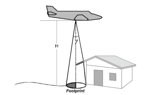
When the laser pulse strikes an edge, part of the pulse continues to propagate and the part incident on the edge registers a return. Thus, multiple returns are achieved usually on vegetation and on surfaces with abrupt discontinuities as edges of buildings.
2.3. Navigation unit
ALS includes a backup measurement record unit, integrated with the GNSS and INS navigation systems [15]. In ALS the georeferencing of the points is totally dependent on the direct georeferencing for the orientation of the sensor and the calculations of the coordinates of each point reached by the laser beam on the surface of the Earth. The final product is the so-called point cloud [12].
3. LIDAR point modeling
A LIDAR point cloud represents the physical surface of the Earth with three-dimensional attributes (X, Y, Z), but with spatial distribution of such non-homogeneous attributes, since they are irregularly separated data. Hence, the modeling of LIDAR points can be given by the generation of a DSM, describing the most relevant elements of the modeled surface [16].
3.1. Grid models
The regular rectangular grid is a model that approaches the real surface through a polyhedron of rectangular faces, of which one of the most important considerations is the spacing between its elements (rectangles), known as fixed spatial resolution [17]. The generation process consists in estimating the Z value (elevation) of each grid point from a set of input samples using interpolation methods [18]. The triangular irregular grid model (TIN) is designed by a polyhedron of triangular faces, whose vertices are the points sampled on the surface [17], and the estimation procedure used in the regular grid is not necessary [18]. In this model, it is relevant to define the best triangulation method.
Observing that a LIDAR cloud is characterized by a high density of points, there is little need to interpolate values to generate DSM, even taking into account that interpolation can degrade the data in regions where there are occlusions caused by the sensor's viewing angle, a very common scenario in urban areas [19].
In order to solve this problem, [20] developed a methodology to generate DSM using the original data values, the coordinates (X, Y, Z) and the pulse intensity. The model was conceived from an empty regular grid whose position and height of each point were projected with the use of the first return. In regions corresponding to "voids" where there is no return of the laser signal, such as on surfaces of bodies of water or in buildings where the signal does not arrive due to the occlusion, a form of filling was necessary. This was done for each empty position in the grid with the average between positions that are the closest to each other, verifying that they had to satisfy a criterion of homogeneity that considered both the difference of elevation and the value of the intensity. At the end, mathematical morphology was used to fill border regions between non-homogeneous areas.
3.2. Distances between LIDAR points
To determine the distances between LIDAR point clouds, the following concepts derived from Analytical Geometry were considered:
3.2.1. Distances from point to point (Euclidean distance)
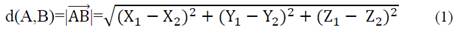
Let A(X1, Y1, Z1) and B(X2, Y2, Z2) be two points of the coordinate system, the distance between points A and B is the vector module, that is:
3.2.2. Distances from point to plane
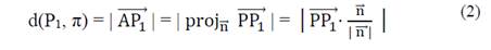
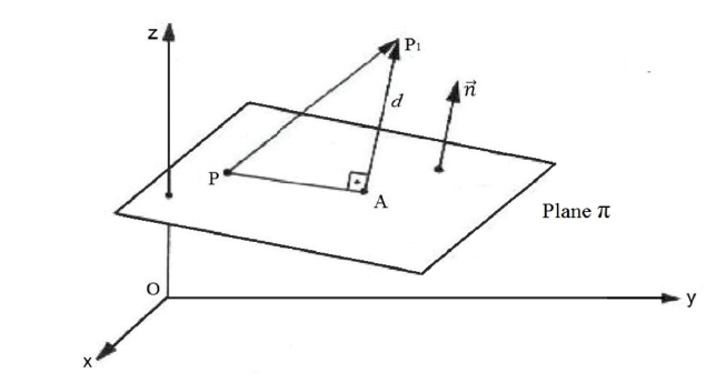
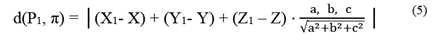
One way of relating the point and plane geometric elements in a cartesian coordinate system in space is by the General Equation of the Plane. Given a point P1 (X1, Y1, Z1) and a plane π, the distance between point P1 and plane π is denoted by d (P1, π) and defined as the shortest possible distance between P1 and a point in the plane. The point of the plane that lies at the shortest distance of P1 is exactly the point at the intersection of the line passing through P1 that is perpendicular to the plane [21], as seen in Fig. 2. The distance from a point (P1) to a plane (π) is defined as the orthogonal projection module of the vector over the normal vector ( n ) to the plane π, denoted as [22]:
As,

E,

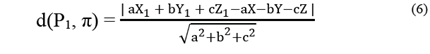
The distance between the point P1 and the plane π is:
Developing,
Since P belongs to the plane π, the General Equation of the Plane is:
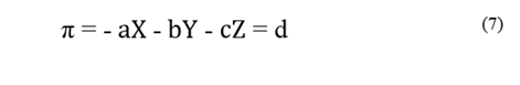
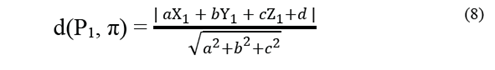
And therefore:
3.3. Digital image processing
3.3.1. Image segmentation
The segmentation of images consists in decomposing an image into its regions (groups of pixels), isolating the objects of interest so that the unnecessary details are extracted and the information of the regions of the image is homogeneous, simplifying and transforming it into another much more representative [23].
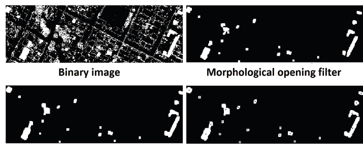
Among the most used segmentation methods, thresholding is a much simpler method due to the ease of its application. The conversion of an image, composed of objects and background with intensity levels grouped into dominant modes, to two pre-set tones from a point is called threshold, as a way to extract the objects of the Fund. The threshold image consists of a binary image, with two levels, usually white and black [23].
3.3.2. Mathematical morphology
Mathematical morphology derived from set theory studies the geometric properties of the image, in which the basic operations of union, intersection, complement and difference are the most used in the definition of morphological operations. The objective is the extraction of geometric structures that can be used for the construction of applied morphological filters in edge detection, segmentation and image enhancement [23].
The basic morphological operations in binary images are Dilation and Erosion. Dilation can be described as the operation that causes objects to expand, used to increase and connect light objects, while erosion produces a reduction of the original image that allows to decrease and disconnect light objects. In practice, dilation and erosion are used together; an erosion followed by a dilation and / or a dilation followed by erosion are known as "opening" and "closing" operators, respectively. The opening separates and eliminates unwanted objects such as image noises (white dots on a black background), while the closing attaches light objects and eliminates small pits. In both cases, this iterative application allows the elimination of specific details of the image without a global geometric distortion of the non-suppressed characteristics [23].
3.4. Image labeling by related components
Labeling is the process of classifying and describing the objects delimited in the segmentation. To this end, consider that the images are formed by connected components that are formed by connected pixels, whose connectivity is composed of all the pixels of the same region that have the same characteristics will have the same value in their levels of ash. Thus, labeling is a procedure for assigning a single label to each object or related component of the image [23] and illustrated in Fig. 3.
4. Materials and survey areas
The LIDAR Systems used are the ALTM 2050 and Pegasus HD500 sensors designed by Optech Inc. The survey area comprises the cities of Ponta Grossa and Curitiba, both in the state of Paraná, Brazil. For Ponta Grossa, data obtained with the ALTM 2050 in 2011 and the Pegasus HD500 in 2012 were available. As for Curitiba, data obtained by the Polytechnic Center of UFPR with the ALTM 2050 in 2003 and with the Pegasus HD500 in 2012 were available.
5. Methodology
The methodology consists of the preliminary correction of errors in the alignment of point clouds and the application of two methods for detecting changes caused by buildings. These changes were classified and quantified using digital image processing techniques and through the analysis of geometric attributes.
5.1. Data preprocessing
The width and area of the strips and the spacing and number of points per strip were identified to calculate mean point density, which was then used to determine the resolution of the regular rectangular grid, the fixed spatial resolution of the DSMs.
5.1.1. Registry comparison of point clouds
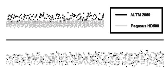
The comparison of cloud records is intended to detect errors in the alignment of different data sets, so that no false alterations are recorded. A systematic error of height could be identified for the ALTM 2050 through the analysis of point cloud distributions in Ponta Grossa. Thus, the systematic error value to be corrected at the Z-coordinate of the ALTM 2050 cloud is 0.22 m or 22 cm, the result of which is illustrated in the profile of Fig. 4.
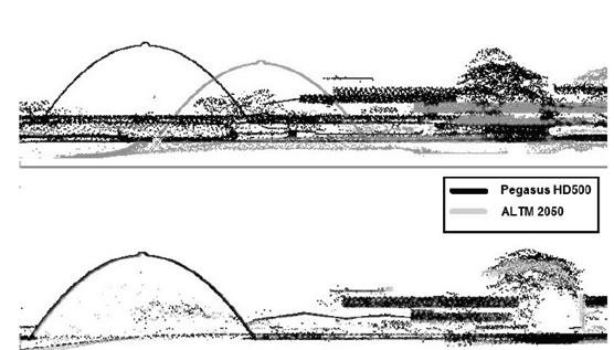
In the Polytechnic Center, the cloud records presented two Geodetic Reference Systems (GRS). To adjust this, the coordinates of the ALTM 2050 frame were transformed to fit the Pegasus HD500 frame. This process was based on the Theory of Transformations among GRS, transforming UTM coordinates, referred to SGR SAD-69/96 to UTM coordinates, referred to SGR WGS-84, whose adjustment can be seen in Fig. 5.
5.2. Methods for detection of variations
The data obtained by LIDAR sensors results in a cloud of points that are randomly distributed in position and elevation. Consequently, these points do not reach the same location in two different surveys. The first method of detection of variations is the regular spacing method, which consists in determining altimetric differences through the subtraction of the DSMs that were generated for the sets of multi-temporal points. Subsequently, a second method - a vector method - is presented. It consists in the determination of the vertical distances between the same point clouds and is characterized as direct for containing the original height information. In order to adapt the results, absolute height differences greater than 2 m and areas larger than 20 m2 were established as criteria for variation identification.
5.2.1. Detection of variations by the indirect method
Regular grids will be generated with no interpolation of height values by using the methodology proposed by [20] for DSMs. This methodology allows using the original values of the LIDAR data, the coordinates (X, Y, Z). Thus, a regular grid was generated for each point cloud of the LIDAR Systems in study (ALTM 2050 and Pegasus HD500). In this way, a code was implemented in the MATLAB software that uses the LIDAR data, stored in ASCII files. This will happen in five basic steps:
a) Determination of the resolution of the regular rectangular grid: grid size was determined by the coordinates of the points (minimum X, maximum X, minimum Y and maximum Y). The fixed spatial resolution was calculated from the mean point density of each survey area.
b) Projection of the points in the grid: each point and its altitude value (Z-coordinate) were projected in the grid.
c) Filling the "empty" cells of the grid: for each empty position in the grid, the existence or absence of elevation values in the neighbor cells will be verified; if any, this grid position is filled with the mean value of its neighbors, which is determined by the elevation values of the first return.
d) Use of mathematical morphology: application of the Closing morphological operator to fill border regions between nonhomogeneous areas.
e) Treatment of regions without information: to fill regions whose pixel values are 0, a window is generated from the raster image obtained in the previous step. This window is determined for each region that is going to be corrected by a manual inspection of the areas. After this, the lowest height value of the specified window is searched, so that this value will be used to replace all the 0 values inside the window, finally filling all the regions and completing the full image with proper height values.
At the end, through a pixel-by-pixel comparison, variations will be detected by the subtraction of the DSMs, which results in an image with lighter tones representing positive variations and darker tones representing negative variations. As for subtractions, the ALTM 2050 DSM is defined as the reference cloud to which the Pegasus HD500 DSM will be subtracted (then defined as the compared cloud), resulting in a third grid, called “grid of differences". To determine the geometry of the objects that were detected as variations, the thresholding process is applied to the images. Afterwards, the Opening and Closing morphological operators will be applied to reduce the areas corresponding to trees. This process occurs in order to identify objects of interest, i.e., the buildings themselves, and to finally obtain, through connected components, the centroids and areas of these objects.
5.2.2. Detection of variations by the vector method
To determine the variations with the vector method, the following criteria were observed:
a) Planes were formed by triangles with the ALTM 2050 cloud as a cloud of reference. Points were formed using the Pegasus HD500 cloud as a compared cloud.
b) Given a point belonging to the Pegasus HD500 cloud, it is determined from its coordinates which of the triangulations of the ALTM 2050 contains the plane coordinates (X and Y).
c) With the establishing of a point (Pegasus HD500) and a triangle (ALTM 2050), the distance will be calculated according to the general equation of the plane. Therefore, since the point of the Pegasus HD500 system is projected in the plane (triangle) of the ALTM 2050 system, the coordinate Z1 of the point P1 is calculated using only (X1, Y1) of the P1, thus:
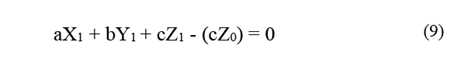
Where P1 (X1, Y1, Z1) is the point projected vertically in the triangle of the ALTM 2050 system, and P0 (X0, Y0, Z0) is the point of the Pegasus HD500 system.
For the determination of the area of the detected variations, its features are segmented according to their continuous geometries, which results in polygons representing the possible buildings, according to their geometric forms.
5.2.3. Classification of the detected variations
Once specific survey areas denominated “experiments” are selected, differences in height in these areas will characterize the variations as new buildings or as demolitions according to positive or negative values, or according to the value types with the highest tendency for each experiment in the two survey areas.
6. Results
6.1.1. Raster method
The grid of differences was represented in an initial image, which became the digitally processed image. The experiments were selected after the identification of the most significant variations in this final image. Fig. 6 shows the image obtained from Ponta Grossa as an example.
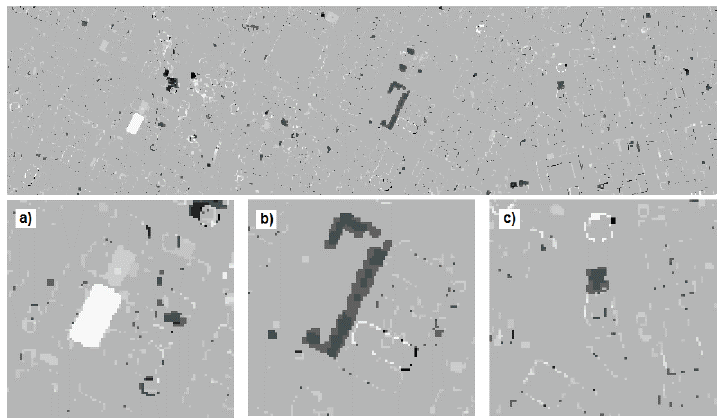
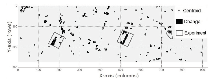
From the image processing of the grid of differences, the objects of interest (variations) and their centroids were recognized. For Ponta Grossa, 414 objects were initially labeled and, after the elimination of objects with areas smaller than 20 m2, 134 variations figured as possible buildings (Fig. 7). At the Polytechnic Center, at the beginning, 890 objects were identified and labeled; after the removal, it totaled 262 variations figuring as possible buildings.
Three experiments were selected for Ponta Grossa with identification of seven objects of interest. As for the Polytechnic Center, six experiments were selected, with 13 recognized objects. With the centroids of these variations, the maximum height differences of each variation were estimated and classified as new buildings or demolitions.
6.1.2. Direct Method
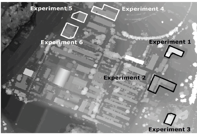
For the development of the vector method, a cut of the LIDAR data from the experiments defined in the raster method was carried out. In the case of Ponta Grossa, these areas are three blocks from the urban area (Fig. 6). As for the Polytechnic Center, they correspond to six singular buildings that are illustrated in the DSM presented in Fig. 8.
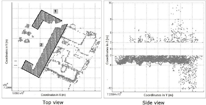
From the results obtained for Ponta Grossa, positive and negative points were detected in all experiments in different quantities and proportions that generally characterize new buildings and demolitions, whereas experiments for the Polytechnic Center show differences in height, mostly positive ones. Fig. 9 shows the results for the experiment B of Ponta Grossa. In the left image, from a top view, two buildings of the court are observed. In this view, the distribution of the points on the edges of the buildings is identifiable. They exemplify the behavior of the return of the pulse in this type of features. In the right image, from a side view, the points are observed with variable heights and dispersed in the positive direction, while in the negative direction they present an important grouping in the height difference of -5 m.
6.2. Verification of the classifications of the variations
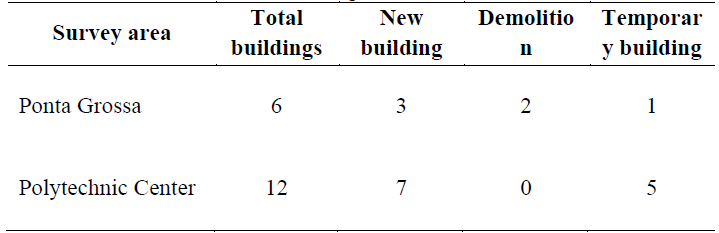
After the classification of the variations detected in buildings, a field verification was found to be timely. Therefore, at this stage, a type of building whose characteristics were not adequate with the predefined categories was found, and a new category called "temporary building" had to be created corresponding to buildings such as tents and greenhouses. Table 1 presents the results of the classification verification.
6.3. Comparison of detection methods
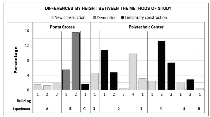
6.3.1. Comparison for height of buildings
In the comparison of the methods by height, it stands out that in Ponta Grossa the percentage of differences is considerably lower for the new buildings and for the temporary building found on site than for the demolished buildings. However, in the case of the Polytechnic Center, the differences have a more dispersed behavior, as shown in Graphic 1.
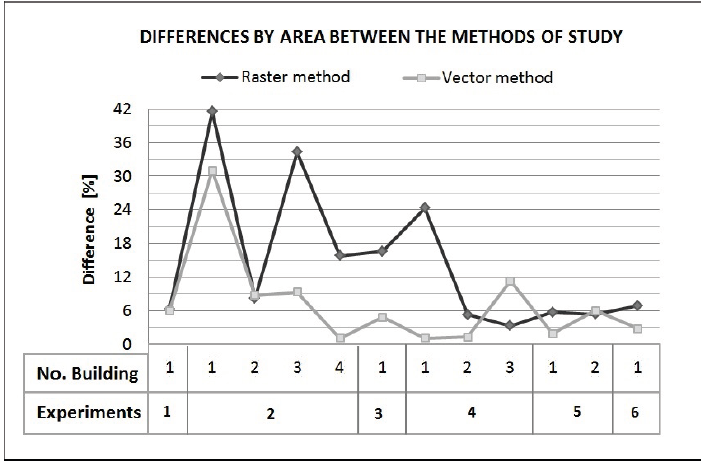
6.3.2. Comparison by building area
From the results it is observed that the variations in area are larger for the Polytechnic Center than for Ponta Grossa, which shows more homogeneous results. It can be inferred that the trend of the differences is slighter for new buildings with respect to demolitions and temporary buildings in the two survey areas.
To ascertain the accuracy of the methods areas, the "true areas" of the buildings in the experiments from the Polytechnic Center were determined. When observing the differences between the methods in comparison to the real areas, there are only two occasions in which the difference of the raster method, which corresponds to temporary buildings, is smaller. Thus, the vector method is more accurate to determine areas of buildings, as shown in Graphic 2.
7. Conclusions
In general, LIDAR sensors have valid altimetric accuracy to detect variations caused by buildings.
When evaluating the accuracy of the methods by comparing the geometric attributes, a discrepancy in the areas obtained in the raster method is evident. This discrepancy does not arise from the detection, but from the processing of the images. It is important to consider that the data calculated by the indirect method show discrepancies because they originate from the height values that result from the process of filling the empty cells in the grids where the laser beam could not reach. Subsequently, the errors derived from the treatment of the images when applying morphological filters further increase the discrepancies, tending to an increase in the areas.
As previously mentioned, the detection of variations with the transformation of data in raster formats is not appropriate to accurately determine shape and size attributes. Thus, it is necessary to search for another technique to automate the determination of areas. However, when comparing the two methods from a practical point of view, a great advantage of the raster method is the optimization of computational time, since the processing of irregularly distributed data such as LIDAR data requires more time than the data processing performed on a regular grid.
The percentage of differences between methods of area determination considerably increases compared to methods based on height differences. It is known that LIDAR data do not accurately detect building edges. This fact can be aggravated when there are trees in the surroundings of buildings, which causes the geometry of the latter to be modified, generating irregular forms. For example: buildings with occlusion problems due to the presence of trees at the edges, where trees can reach up to half the roof of a building. In this case, the tendency in the calculation of areas is overestimation. Therefore, to accurately determine areas in buildings with occlusion problems, it is recommended to remove the vegetation by filtration, hoping that this removal, performed by computer programs, will bring considerable improvement in the computation automatism of building attributes.
Cross-over flight planning is also an option to increase information on buildings. LIDAR surveys with several flight lines in different directions, regardless of differences in parameters, may help to fully cover the regions where the laser beam does not reach the targets and thus obtain a wider coverage of the buildings.
On the subject of classifications, the effect of the methods that automatically perform processes of classification of the variations from buildings are reduced by the need to perform field surveys.
This necessity of carrying out field surveys ends up minimizing the demand to find methods that automatically perform the processes of classification of variations from buildings.
With respect to the total automation of procedures of detection of buildings in urban environments, a dynamic advance is observed in technological tools that include algorithms of classification of LIDAR point clouds, in such a way that each time is less the intervention of the user. However, there are cases as temporary constructions, presence of occlusions and / or dense vegetation, where such algorithms do not have the ability to discern the characteristics of the elements in study, for example, classify a tent or awning as a temporary construction and not as an actual building or distinguish a demolished building of appearance of high vegetation, are tasks that the user could do, by the simple experience and common sense of human perception.

