


 Spanish (pdf)
 Article in xml format
 Article references
 Send this article by e-mail
 Cited by SciELO
  Cited by Google
  Similars in
SciELO
Similars in
SciELO  Similars in Google
 Permalink
1. Introduction
Precision agriculture (PA) can be defined as the use of agricultural techniques based on information technologies for the treatment of spatial variability of soil properties and characteristics from determined area [1].
The rising demand for variability management of soil and plant properties in the field is allied with availability and adoption of PA tools and technology. Together with geospatial tools, using global navigation satellite systems (GNSS) and geographic information systems (GIS), it becomes a highly reliable tool for the spatial characterization of soil properties [17]. However, there is still an obstacle about techniques for data collection on soil properties in a quick, efficient, and accurate way [25].
The method traditionally used for soil sampling may become unviable due to the expensive field work and laboratory as a function of the high number of samples. Moreover, the traditional method is negatively impacted by the higher cost and time to obtain the results, and hence in the subsequent creation of reliable thematic maps, becoming necessary to seek more efficient and advanced methods for collecting and processing these data [15,2].
According to Mulla [18], the future will require massive data collections and analysis on a scale considered not feasible at present, involving stationary or mobile sensors that can accurately measure different plant characteristics in real time. Sensors capable of mapping some soil properties are already available to the farmer. This type of equipment allows performing soil pH sensing in high resolution through antimony ion-selective electrodes [22].
Aiming at this cost saving and searching for reliable results, geostatistics is a technique that works on the characterization of the spatial dependence or not of the elements under analysis, when supplied with a mass of data with aggregated geospatial information. In PA, this technique becomes very useful in planning and mapping the variability of soil physical and chemical properties, interpolating values of these attributes to non-sampled sites, using a mathematical model named kriging [20,2], enabling the creation of thematic maps that characterize the spatial distribution of properties in an area, becoming a basis for the farmer to make decisions on soil management and farming.
The aim of this study was to characterize the magnitude of the spatial variability of soil pH sampled by two different methods used in PA, in order to fit semivariograms from different methods and models, thus obtaining isochore maps interpolated by kriging more reliable, being possible to observe differences among the sampling methodologies.
2. Material and methods
The experiment was performed in the municipalities of Guarapuava and Cantagalo, both in the state of Paraná, located at the geographic coordinates 25° 31’ 22.60” S and 51° 30’ 16.46" W for the Cupim Farm (A1) with an area of 60 ha, and coordinates 25° 16’ 52.25” S 52° 6’ 12.89" W for the Juquiá Farm (A2), with an area of 20 ha. The climate of the region is Cfa, according to Köppen classification. The areas are cultivated under crop rotation of soybeans, oats and maize. The soil of the study areas is characterized as inceptisol, with prominent A horizon, smooth undulating relief and basalt substrate [11], with a textural class varying from clayey to very clayey.
For the determination of soil pH values for both areas, two different methods were used in relation to their determination principles: i) collection in grid sampling, ii) collection through on-the-go soil sensing.
Grid sampling of one point per hectare (100 x 100 m) were developed in both study areas in order to collect the pH, which were correctly georeferenced with the aid of a GNSS signal receiver with high-precision differential correction. Each sample was withdrawn at a depth of 0-20 cm using an soil auger. At each georeferenced point, 11 to 15 subsamples were collected randomly at a radius of 3 m from the center point. These subsamples were homogenized properly generating a single sample representative of the sampling point. The soil samples were sent to the Coodetec soil analysis laboratory, where the necessary chemical analyses were performed.
The second sampling method, also performed in both areas, used an on-the-go sensor for soil pH of the Veris PMC® platform ("P" - pH, "M" - organic matter and "C" - apparent electrical conductivity).
Schirrmann et al. ([22]) describe Soil pH Manager™ which is a module of the Mobile Verisme Platform (SMP) as a sensor that measures soil pH in direct contact with the samples when the equipment is in motion. This sensor is divided into three parts: i) hydraulic system for routing of soil samples, ii) pH electrode measurement system, iii) washing system with distilled water.
During the course of sampling, the hydraulic system is activated so that a metal structure penetrates the soil to a defined foot depth for sample removal. The collected samples are suspended by the hydraulic actuator so that they come in contact with the antimony electrodes. The up and down movement of the soil sampler (hydraulic system) is driven by a proximity sensor. PH is measured in untreated and naturally moist samples. The pH value of the samples is calculated as a function of the average voltage that the electrodes emit to the system that performs the voltage conversion to pH values.
The measurement time of each sample is on average from 7 to 25 s. After pH measurement the electrodes are washed with distilled water stored in the upper part of the equipment by two nozzles located next to each electrode.
According to Schirrmann et al. [22] and in accordance with Veris Technology's calibration recommendations, calibration of the sensor's antimony electrodes is done by a two-point calibration using standard solutions of pH 4 and 7 at the beginning of each experiment. In this calibration the electrodes were inserted into the buffer solution and it was gently shaken for 30 sec to a steady state. The calibration process lasts around 2 min.
The sensor was tractioned by a tractor with an average forward speed of 9 km.h-1, which ranged 30 m spaced transects in the entire area. The density observed for the use of sensor averaged 200 points per hectare. The tractor also had an integrated satellite navigation system, which provided a correct parallelism among transects and the georeferencing of the points sampled by the equipment.
In order to characterize the spatial dependence of the soil pH in both study areas referring to the two soil sampling methodologies, geostatistical analyses were performed by classic and robust semivariograms. The classic semivariogram was estimated according to eq. (1):
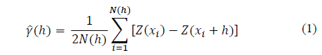
Where: N (h) is the number of experimental pairs of observations Z(xi) and Z(xi + h) separated by a distance h. The semivariogram is represented by the graph ("γ ") ̂"(h)" versus h. From the fit of a mathematical model to the calculated semivariation values (("γ “) ̂"(h)"), the coefficients of the theoretical model were estimated for the semivariogram called: nugget effect (C0), sill (C0 + C1), and range (a), as described by Vieira et al. ([24]).
According to Cressie and Hawkins [7], the robust estimator of semivariogram values is less susceptible to the influence of mass data values than the classic estimator. Thus, the robust estimator is described by eq. (2).
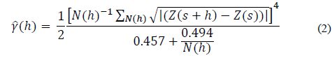
The robust estimator assumes that the differences Z(s+h) - Z(s) are distributed normally for all pairs (s+h, s). The transformation of the square root of differences is shown as having moments similar to those from the normal distribution and the denominator of the equation is the bias correction [9].
The fitting semivariogram models were selected according to the ordinary least squares (OLS) and weighted least squares (WLS) estimated by classic and robust mode and maximum likelihood (ML) and restricted maximum likelihood (REML) using the classic estimator. For all methods, the spherical, exponential and Gaussian models will be tested, totaling 18 semivariograms for each variable. For the choice of semivariogram fitting methods and models, data validation will be considered (Fig. 1) [8,9], assuming the stationarity of the intrinsic hypothesis of omnidirectional behavior. [2]
Validation is an error estimation technique that compare predicted values with sampled ones [12]. The sample value, at a certain location Z(si), is temporarily discarded from the data set, and then a kriging prediction is performed on the location, using the remaining samples.
Some values will be very useful for the best method choice, such as: Mean error (ME), the standard deviation of mean error (SDME), reduced mean error (RE) and the standard deviation of reduced mean errors (SDRE). Eq. (3) represents the mean error by validation (ME):
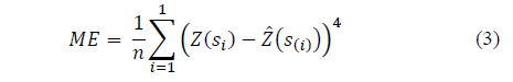
Where n is the data number, Z(si) is the value observed at point si, and

 is the value predicted by ordinary kriging at point si, excluding the observation Z(si) (Faraco et al., 2008).
The reduced mean error (RE) is defined by eq.(4) :
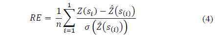
Where
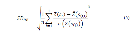
 is the standard deviation of kriging at point si, excluding the observation Z(si). The standard deviation of reduced errors (SDRE) is obtained from Eq. (5) :
According to Cressie [6] and McBratney and Webster [16], the models can be evaluated by reduced mean error (ER), standard deviation of mean errors (SDME) and standard deviation of reduced errors (SDRE).
As closer to zero the average difference among the values, the best the estimator. The selection criteria based on validation should find the value of ME and RE closest to zero, the value of SDME should be the lowest, and the value of SDRE should be closest to one.
The choice of the best theoretical fitting model of empirical semivariogram of pH for each area and for each sampling method was performed, considering some criteria based on validation, such as the mean error (ME) and the reduced mean error (RE) closest to zero, the value of standard deviation of mean error (SDME) should be the lowest among the methods, and the value of standard deviation of reduced mean error (SDRE) should be the closest to one. Thus, the fitting model and method of semivariogram that met the highest number of validation requirements would be used. However, if this is not met, the model and the method where the sill (the sum of the nugget effect plus the contribution) is closest to the variance will be used as the decision criterion ([10]). According to Webster and Oliver [27], the sill value must be close to the value of data variance if the semivariogram cloud has a sill.
After fitting the mathematical models of semivariogram and the conjugation that promoted the best validation statistics, the data interpolation observed by ordinary kriging with an interpolation radius equivalent to the range of the fitted semivariogram was performed in order to allow prediction of pH values at not sampled locations [13]. For modeling purposes of the experimental semivariograms, an omnidirectional pattern was assumed.
The georeferencing of the area was performed based on the geographic coordinates obtained by a differential GNSS signal receiver in the demarcation phase of sampling points. The data processing for the geostatistical analysis was performed in the R statistical software, through the geoR library [19], and isochore maps were generated in ArcGIS 10.0 software.
3. Results and discussion
The results referring to the descriptive statistics applied to the pH data collected through the two different methodologies are described in Table 1. A difference/amplitude of the maximum and minimum pH values is observed through on-the-go soil sensor in the order of 1.6 pH unit (5.2-6.8) referring to sampling for area A1. In contrast, this difference was 2.25 pH units (5.15-7.40) for area A2.
Based on the analysis of descriptive statistics presented in Table 1, it can be observed that the averages of pH values sampled by grids and sampled by sensor in both areas were different.
Table 1. Descriptive statistics of pH sampled by grid (pH grid) sampling and by on-the-go soil sensor (pH sensor
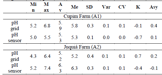
Min - minimum value of the variable, Max - Maximum value of the variable, Av - Averange, Me - Median, SD - Standard deviation, Var - Variance, C.V. - Coefficient of variation, k- Coefficient of kurtosis, Asy - Asymmetry.
Source: The Authors.
This can be explained mainly because the on-the- go soil sensor obtains a larger number of samples than the traditional method. The pH values observed by the sensor were higher than the values obtained by the traditional method in area A2.
Chirmman et al. (2011) reported an estimate of pH values by on-the-go soil sensor higher than the data from the laboratory for soils of Germany. This sensor behavior was not observed for area A1.
The results from the CV analysis of both pH sampling methods were lower than 10%, so that the scatter of values around the mean is considered homogeneous, according to Warrick and Nielsen [26]. However, it should be emphasized that the occurrence of highest and lowest values of pH in the areas was not characterized spatially, being necessary to use a geoestatistical analysis of these values.
Based on the methodology for determination of geostatistical analyses, it was possible determine the parameters (C0, C0+C1, a) of semivariograms (Tables 2,3) fitted by different methods and models for characterization of spatial dependence of pH obtained by different sampling methods in both study areas.
Table 2 Methods, models and estimated parameters of experimental semivariograms for the pH sampled by grid and by sensor in the Cupim Farm (A1)
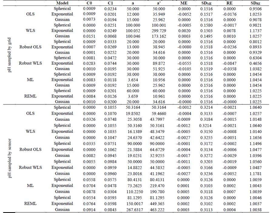
C0 - Nugget effect, C1 - Contribution, C0+C1 - Sill, a - range, a'- practical range, ME - Mean error, SDME - Standard deviation of mean error, RE - Reduced mean error, SDRE - Standard deviation of reduced mean error, WLS - C - Weighted least squares classic estimator, ML - Maximum likelihood, OLS - R - Ordinary least squares robust estimator, REML - Restricted maximum likelihood, Sph - Spherical, Exp - Exponential.
Source: The Authors.
Table 3 Methods, models and estimated parameters of experimental semivariograms for the pH sampled by grid and by sensor in the Juquiá Farm (A2)
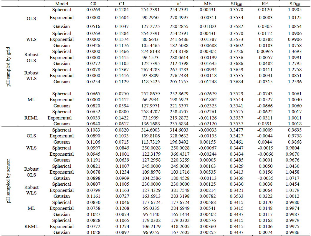
C0 - Nugget effect, C1 - Contribution, C0+C1 - Sill, a - range, a'- practical range, ME - Mean error, SDME - Standard deviation of mean error, RE - Reduced mean error, SDRE - Standard deviation of reduced mean error, WLS - C - Weighted least squares classic estimator, ML - Maximum likelihood, OLS - R - Ordinary least squares robust estimator, REML - Restricted maximum likelihood, Sph - Spherical, Exp - Exponential.
Source: The Authors.
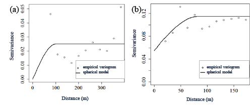
Based on the validation criteria, for the pH data referring grid sampling method (Tables 3,, semivariograms (Fig. 1 a , 2 a) were obtained for both areas fitted using the robust WLS method, indicating the spherical model (Fig. 1 a ) and exponential model (Fig. 2b). After the theoretical fitting, it was possible to observe that the range (a) determined for both areas ranged from 92 to 100 m. The range (a) is important to determine the spatial dependency threshold of the attribute with other points, which can also be comprehended as the threshold distance at which a sampled point correlates with the points around it, indicating that points sampled in a radius equal to the range tend to be more homogeneous [6,20].
Source: The Authors
Figure 1 Semivariograms of pH sampled by grid (a) and sampled by on-the-go soil sensor (b) on the Cupim Farm area (A1).
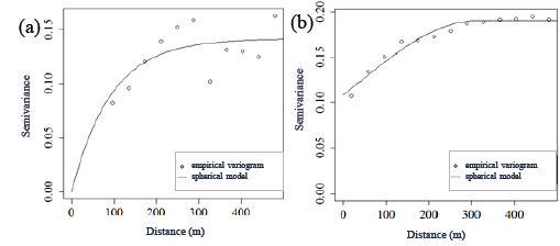
For the sampling method by on-the-go soil sensor, the experimental semivariograms allowed fitting through the REML (Table 2) and OLS method (Table 3), and it was evidenced that the spherical model was satisfactory according to validation criteria for both studied areas (Figs. 2 b , 3b). However, the ranges (a) found for semivariograms referring to pH sampling by sensor (Figs. 2b, 3 b) were 81 m and 364 m, respectively. According to Souza et al. [23], changes in range values (a) may be related to management techniques applied in soil, which may be distinct for different areas.
Source: The Authors.
Figure 2 Semivariograms of pH sampled by grid (a) and sampled by on-the-go soil sensor (b) on the Juquiá Farm area (A2).
The semivariograms referring to grid sampling method (Figs. 2 a-3 a) show C0 values equal to 0 (Table 2). However, for semivariograms representing the semivariance of pH data collected by sensor (Tables 2, 3), the values are equal to 0.065 and 0.183 for areas A1 and A2, respectively. According to McBratney and Webster (1986), the nugget effect (C0) is a semivariogram parameter that can indicate how much the data variance cannot be explained for a distance smaller than the radius among samples and for measuring errors. However, it is not possible to detect which of these factors has greater weight in the discontinuity of variance values.
Sana et al. ([21]) reported that determining the range of semivariogram fitted according to a theoretical model is essential, since it allows interpreting how far the prediction of a value is influenced by a sampled point in another nearby place. These authors found in their study a low CV for the traditional sampling method of pH, for a grid sample of 0.64 points per hectare, and later generated pH maps through kriging, observing that the best fitting model of semivariogram for pH data was the spherical model, which corroborates with the results obtained in this study for the traditional method of pH determination.
Cherubin et al. ([3]) reported that a reliable fitting model cannot be generalized to evaluate the variability of attributes for a latosol in Rio Grande do Sul, Brazil, because the variability of each attribute is conditioned to intrinsic and extrinsic factors from each analyzed area, in which the semivariogram referring to each analyzed attribute and area can be fitted by different theoretical models.
In this study, it was observed that the range of semivariogram was changed, with higher values due to the determination method of pH values (Figs. 1, 2, Tables 2, 3). According to Corá et al. ([4]), the prediction quality of values in non-sampled points is strongly influenced by range values, and the ordinary kriging results are more reliable when higher range values are adopted, approaching the field reality on thematic maps referring to the spatial distribution.
After the best method and fitting model of each semivariogram was chosen, the ordinary kriging of pH values was performed, making it possible to generate thematic maps of the spatial distribution of pH sampled by grid and sampled by on-the-go soil sensor. To provide a visual comparison of maps, seven division classes of pH values were used for both study areas (Figs. 3-4).
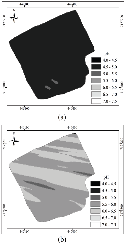
In Figs. 3 a,4 a, the maps of the spatial variability of pH on area A1 are observed, where it is noted a difference in pH values between the soil sampling methods performed in the area. Observing Fig. 3a, it can be observed that the pH values of the area ranged from 5.5 to 6.0, and the map is mostly darkest gray (whose pH value is 5.5), totaling an area of 18.42 ha. By analyzing Fig. 3b, it is noted that the map represents spatial variability greater than the map of Fig. 3a, and that the value of 6 pH units corresponds to a significant area of the map (11.49 ha).
Source: The Authors.
Figure 3: Grid sampling (a) and on-the-go soil sensor (b) of the area belonging to the Cupim Farm (A1).
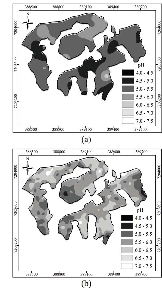
Figs. 4 a, 4 b show the spatial variability maps of the pH from A2 referring sampling methods by grid and by sensor. From the analysis of Fig. 4 a , it can be realized that a large part of the area had pH values equal to 5.5 (darkest gray), representing an area equal to 39.51 ha. In Fig. 4 b , it was observed that a large part of the terrain showed light grey color (pH of 6.5), totaling an area of 29.28 ha. By Fig. 4 b , it is possible to observe a greater variation of pH in relation to Fig. 4 a , in which a greater number of pH classes cannot be observed visually.
Source: The Authors.
Figure 4 Grid sampling (a) and on-the-go soil sensor (b) of the area belonging to the Juquiá Farm (A2).
In Figs. 3b, 4b are shown points of higher pH values that were not observed in grid sampling (Figs. 3 a, 4 a), but it was not possible to observe points of lower pH values through maps of sampling by sensor, which were detected in the sampling maps by soil auger (Fig. 4 a ). A possible explanation for this difference in the readings using the sensor is that the sample was collected possibly more accurately in the pre-established layer, which in our case was 15 cm depth. Thus, the long-time under no-till system in the area (about 15 years) contributed to the existence of a layer with higher pH.
Outliers were observed in the spatial distribution of pH among the results obtained by on-the-go soil sensor (Fig4 a ) and by grid sampling (Fig4 a ), performed at common points for both methods. In Fig4 a , it is verified that pH values are higher than the value informed by laboratory analyses (Fig4 a ), indicating that the obtained results were influenced possibly by some external factors.
The variations in the pH values obtained by sensor and values determined in the laboratory can be explained, according to Chirmman et al. (2011), by the interference of external factors, increasing the reading error of the on-the-go soil sensor in relation to the traditional method of laboratory analysis. These authors emphasize that a best calibration of the equipment is needed, but also make reservations to laboratory errors, in which the mixtures of soils from different layers and locations to compose a single sample can mask the result, besides the number of samplings performed for each determination method.
Corassa et al. [5] analyzed the correlation of soil electrical conductivity by on-the-go soil sensor, and observed that this process of determining real-time soil properties requires specific care, such as calibration for each type of soil and crop. However, when there is a high spatial resolution, i.e., a high number of sampling points, associated with oriented or traditional sampling, the use of sensor can lead to satisfactory results and savings in the application of inputs.
In Figs. 3b, 4 b, it was observed that the maps generated through interpolated data from on-the-go soil sensor are more sensitive to spatial variation of pH than maps generated through pH data determined by grid sampling method and from laboratory analyses (Figs. 3 a, 4 a). Cherubin et al. [3] reported that the reduced grid sample improves the accuracy and the variability characterization of soil chemical properties through thematic maps. Souza et al. [23] studied the intensity of sampling in red latosols in relation to the accuracy of values estimated by kriging and reported that the number of sampling points influenced the prediction of values for points not sampled by kriging, where the error was increased whether the number of samples was lower than 100. These authors also emphasize that a minimum of 100 samples is required for geostatistical analysis, in order to prepare thematic maps to guide agronomic management.
Kerry and Oliver [14] also recommend that practitioners of PA should not use the kriging process with variograms calculated based on a low sampling number and with large distances among points, since they may lead to misinterpretations in the application of agricultural inputs and pesticides at variable rate, masking the benefits from the PA. Kamimura et al. [13] conclude that the kriging method for point interpolation in non-sampled regions is a valid process.
Schirrmann et al. [22] report that prediction errors of 0.1 pH units may result in an under or over application of 400 kg.ha-1 of CaO, according to local liming recommendations, which may result in losses for the producer. Although these authors have been successful in correlating pH soil values in northeastern Germany through on-the-go soil sensor and values determined by laboratory, these authors also report that calibration process of the equipment is extremely important, reducing errors in the application of inputs in the area and production costs.
The use of kriging, after fitting semivariograms, proved to be a very valuable process, allowing a best prediction of pH values by on-the-go soil sensor. These information become very useful for the producer, assisting him in the decision making, delimitating management zones in order to perform processes of input application at variable rate, which would not happen whether the map generated from pH values was obtained by traditional analysis.
4. Conclusions
The semivariograms allowed characterizing the magnitude of the spatial variability of pH sampled by grid and by on-the-go soil sensor.
The test of different methods and models allowed identifying which of them best fitted the variable in each sampling method studied.
The interpolation by kriging allowed generating isocolors maps, providing the observation of spatial variability.
The geostatistical analysis of both different sampling methods of soil pH allowed suggesting that the on-the-go soil sensor provided a best representation of soil pH variability in both studied areas and that the sampling number has limited the visual representation of soil pH variability when it is determined by grid sampling method.

