


 English (pdf)
 Article in xml format
 Article references
 Send this article by e-mail
 Cited by SciELO
  Cited by Google
  Similars in
SciELO
Similars in
SciELO  Similars in Google
 Permalink
1. Introduction
Over the years and with the constant climate change and population increase worldwide, the demand for water resources has also increased and with this, the design and implementation of hydrological modeling used as a software tool both aggregated and distributed, which are subject to multiple variables such as discharge, velocity, Manning coefficient, wet-dry limit, type and size of mesh, and some others, on which the success of modeling depends.
The correct characterization of these parameters and especially, the roughness or Manning coefficient allows performing more precise calculations of velocity, discharge and water depth in each cell of discretization of the basin, which represents a hydrograph of output more accurate with reality. However, taking into account that most of hydraulic and hydrological modeling take as reference a hydraulic Manning, it is pertinent to carry out studies of the distribution and simulation of natural hydrological processes such as rainfall, runoff, moisture soil and / or evapotranspiration, mainly in basins that lack of information of said processes or where this is limited; as well as the calibration of the same for its application in hydrological studies, in which it is considered that this coefficient is affected by the low heights of the sheet of water in the areas of contribution of the basin, causing the presence of vegetation to influence in the hydraulic resistance of the runoff flow in an important way [1] and making it fundamental to the proper determination of these values for distributing hydrological modeling, despite the strangeness of carrying out the calibration from another model, such as the HEC-HMS software, which is widely recognized worldwide [2]; what has its reason for being in the non-instrumentation of the basins under study.
Based on these considerations, this work will result in reference values for the Manning coefficient "n" of hydrological type for some of the most common vegetation coverings, such as grasslands and forests; This will be carried out by generating the output hydrograph for the data corresponding to each of the rural basins not instrumented in the study and later, it will be compared with the hydrogram generated by the Iber software for the same basins. For this purpose, the Manning coefficient will be varied as input data in the Iber software until obtaining a very similar output hydrograph to that provided by HEC-HMS.
This is done taking into account that the basins under study are basins lacking of instrumentation and, therefore, there is no information on observed discharges that allow the calibration of the roughness parameter and with this an adequate hydrological modeling in the non-instrumented rural basins, and that this is depends on a good calibration during the simulation.
2. Statement of the problem
When an engineering project is being carried out in the area of hydrology, to determine the behavior and generation of discharges caused by rainy processes, hydrological modeling is used, which is implicit in a degree of uncertainty, associated with the parameters and input data, as well as the methodological calculation and hydrological software implemented.
In the mathematical modeling of rainy systems and processes, aggregated and distributed models are available, where their selection depends on the complexity of the project, its purpose, the extension in the basin area, the available information and the tools of support software available to specialized personnel. Once the type of hydrological model has been selected, the program that allows carrying out its implementation and the calculation of the basin is defined, starting from the given parameters and the form of construction of the model in the program.
In our environment, aggregate modeling is the most usual since its application is more practical and requires less information compared to distributed models, so it does not consider the events inside a basin and its product is an output hydrograph; while the distributed models imply a greater knowledge of the physical characteristics of the basin and a great computational requirement, since in this type of models the roughness coefficient is more sensitive to the variation of various parameters, such as the height of the vegetation, the draft height and its influence on hydraulic flow and the variation of the roughness, which allows it to be considered in the evaluation of the behavior of the flow before a rain event [1]. Based on the above and taking into account that there is great difficulty in determining the roughness coefficient "n" because there is no exact method for estimating this term [3], this research will focus on calibration of the roughness by Manning's "n" coefficient, which is fundamental to be able to calculate in a more accurate way those variables that have an impact on the resulting hydrograph of the basin, such as discharge, velocity and draft data in each discretization cell of the basin, because although there is ample information of reference values for hydraulic modeling of this coefficient, in terms of hydrological modeling there are no references, so the applicability of the same hydraulic values to hydrological modeling is inadequate [1].
The distributed hydrological model to be used will be the Iber software, which is a hydrodynamic model that solves the two-dimensional Saint Venant equations that works using a finite volume scheme. The results obtained will be compared and calibrated with the results obtained from the HEC-HMS software, which is software that has worldwide recognition and validation [2]. It will be compared with this software because the basins under study will be basins lacking of instrumentation and, therefore, there is no information on observed discharges that allow the calibration of the roughness parameter. From the aforementioned, this work aims to answer the following question: Is it possible to determine the roughness coefficient "n" of Manning in non-instrumented rural basins for different coverages from the comparison of the hydrographs resulting from the hydrological models IBER and HEC - HMS?
3. Manning’s roughness coefficient
“The roughness coefficient "n" is a parameter that determines the degree of resistance offered by the walls and bottom of the contour to the flow. The rougher or rougher the walls and bottom, the more difficult the water will have to move. This parameter has been very studied by many researchers in the laboratory so there are different formulations” [2].
Many authors treat the affectation of this parameter in the flow from a hydraulic approach, but in several of its conclusions, they affirm that the values obtained may not be adequate for a hydrological approach [1].
The value of "n" is very variable and depends on several factors that must be chosen according to the design conditions. The factors involved in the determination of the roughness coefficient of Manning are the roughness of the surface, the vegetation, the irregularity of the channel, the alignment of the channel, the sedimentation and erosion, obstructions, the size and shape of the channel, the level and discharge, seasonal change, suspended material and bed load [4]
3.1. Manning coefficient in hydrological scenarios
The flow conditions in a hydrological scenario vary considerably with respect to a hydraulic scenario, basically due to the fact that the conditions of the height of the sheet of water or draft [5].
Faced with this, Caro [1] collects various conclusions that have reached multiple authors in relation to these approaches and according to which some say that an increase in the height of roughness will be represented in an increase in the depth of flow; while others declare that for flow heights much higher than roughness heights, the roughness coefficient that represents the roughness of the bottom and of the vegetation can be kept constant before changes in the draft. However, if this parameter remains constant in time different inconsistencies in the distribution of a flow can be generated.
In natural channels, the roughness has two important components: grain (irregularities of the walls or size of the bottom sediment) and the roughness of the vegetation [1]. For shallow drafts, where the height of the vegetation remains not submerged, the roughness decreases with the increase in the height of flow. When the submergence begins, this is understood as equalization of the height of vegetation with the height of flow or draft, there is an increase in roughness with respect to the draft increase; however, immediately afterward, when the draft continues to increase, the roughness undergoes a significant gradual decrease [5].
Roughness plays a fundamental role in the model, and it is essential to fix it before you can launch the calculation. In Iber for example, without a reference roughness value assigned to the mesh, it is impossible to perform any kind of simulation [1]. This roughness is assigned through the Manning’s roughness coefficient that analytically comes from the eq. (1)-(3) [6].
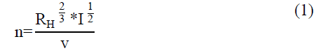

Where I am the energy gradient slope, v the average velocity, RH the hydraulic radius, Pm the wetted perimeter y A the surface or area.
However, the determination of this coefficient is not limited to the application of the eq. (1), since there are various factors such as inaccuracies and construction errors that alter the regularity of the channels, or for the case of water bodies, rivers, streams, etc., elements such as geometric irregularity, different degrees of vegetation cover, land use and land geomorphology; which are considered complex variables to quantify and make accuracy in the calculation of roughness coefficients difficult [6].
4. Hydrological models used
4.1. Hydrologic Modeling System (HEC-HMS)
In HEC-HMS (Hydrologic Engineering Center's Hydrologic Modeling System) is a rain-runoff model, developed by the Hydrologic Engineering Center HEC the U.S. Army Corps of Engineers USACE; designed to simulate the runoff hydrograph that occurs at a certain point in the fluvial network as a consequence of a rain episode [7].
The hydrological models in this program as described Morris [8] are mainly made up of a basin model, a control model, and control specifications.
4.2. IBER model
Iber is a two-dimensional mathematical model developed by the Grupo de Ingeniería del Agua y del Medio Ambiente, GEAMA (Universidad de Coruña), by the Grupo de Ingeniería Matemática (Universidad de Santiago de Compostela), by the Instituto Flumen (Universidad Politécnica de Catalunya y Centro Internacional de Métodos Numéricos en Ingeniería) and promoted by the Center for Hydrographic Studies of CEDEX, based on two already existing numerical modeling tools, Turbillón and CARPA; which are based on the finite volume method[9].
4.2.1. Hydrological modeling in IBER
Iber includes some features that enable the computation of rainfall runoff transformation and therefore, make possible to use Iber as a distributed hydrological model based on the 2D shallow water equations [10].
The present version of Iber does not include a groundwater flow module and therefore, the base flow component is not considered in the model. This limits its applicability as a hydrological model to short and intense rainfall events in which the contribution of the base flow to the total discharge is less relevant than the surface flow contribution. [10].
Likewise, in the tools used to carry out hydrological modeling, IBER has a decoupled hydrological discretization (DHD) scheme, which is an important selection to obtain a more stable hydrological calculation, as well as the definition of the wet-dry limit, the type, and size of the cell and the Fill Sinks tool. The proper use of the above parameters and tools leads to more reliable results.
Considering the existence of instabilities in hydrological calculations, a new numerical scheme called decoupled scheme was added in the most recent versions of Iber and as a complement to the first and second order schemes that were already available [11].
This new scheme has the purpose of solving some instability produced for hydrological calculation cases with very small discharges [1]. For hydraulic calculations, especially with large drafts and with regime changes, instabilities can be generated in the same way [2].
According to [2] the main difference between the decoupled scheme and the first and second order schemes is the way to discretize the Saint-Venant equations. However, for the implementation of this numerical scheme, some changes were made such as the elimination of the pending source term of the fund, the calculation of a new source term that depends on the slope of the free sheet and redefining the numerical flow based on a discretization centered and off center.
The dry-wet threshold is a variable that indicates the limit height of draft above the Iber considers a finite element as wet, which will improve the performance of operations within the program, for those elements that are recognized As dry, no calculations will be made, thus decreasing the duration of the modeling [2].
Iber incorporates the following three wet drying methods: Normal or default drying, Strict drying and hydrological drying [2].
Normal or default drying: The one that Iber uses by default and that allows negative drafts in order not to increase the ∆t. It is useful for drafts not too small where the instabilities would increase by this permissiveness in terms of negative drafts [2].
Strict drying: This method is the most accurate and with less instability available to Iber since it does not allow negative drafts, but it increases the calculation times since they decrease the ∆t [2].
Hydrological drying: The most recent, does not allow negative drafts without the need to decrease the ∆t too much, which would increase calculation times. The method scales the output discharges in each element and for each time increment. If the drafts are low enough, the method strongly avoids instabilities [2].
The tool "Fill Sinks" was initially implemented in the version 2.0 of Iber with the purpose of filling the depressions found in the MDE (Digital Elevation Model), from the modification of the height of that pixel, thus allowing the flow of the water, since there is a continuous slope towards the outlet of the basin [2].
This option is located on the route Data> Problem Data> General> General Options> Activate the display tab> Activate the option "Fill Sinks".
The mesh is a set of contiguous cells that allows representing in a discrete way the domain of a problem to be solved numerically, which for the particular case of Iber turns out to be a surface [2].
The reliability of the numerical solution obtained depends on the quality of the generated mesh. The quality criteria used depending on the chosen numerical method and the type of problem to be solved. On the other hand, the type and size of the mesh are what determines the calculation time, so choosing these variables correctly is fundamental [2].
Mesh generation, both structured and unstructured, can sometimes generate certain instabilities or depressed areas where water accumulates. Some of these depressions are the result of errors in the data introduced during the surface generation process, while others represent real topographic features, such as quarries or natural potholes [1].
5. Hydrological modeling
In order to address the problem described, a procedure was established to determine the value of the roughness coefficients with a hydrological character for a vegetation cover of forests and grasslands, which is based on the variation of the Manning coefficient as input parameter in the Iber software and the comparison between the output hydrographs of the same and the modeling carried out in HEC-HMS for the same basin.
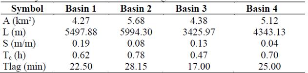
5.1. Morphological study of the basins
Starting from the digital elevation model obtained from the ALOS Sensor Palsar Satellite, whose resolution is 12.5 X 12.5 meters, the topographic parameters of the basins under study were obtained; from which, and with the help of the Hec-GeoHMS extension of ArcGIS 10.2, the watershed divide was defined, as well as the slope of the channel (S), the maximum length of flow (L), the afferent area (A), the concentration-time (Tc) and the lag time (Tlag) of the basin.
5.2. Concentration-Time (Tc) and Lag Time (Tlag)
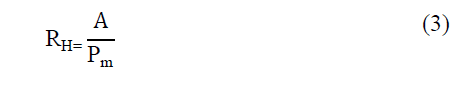
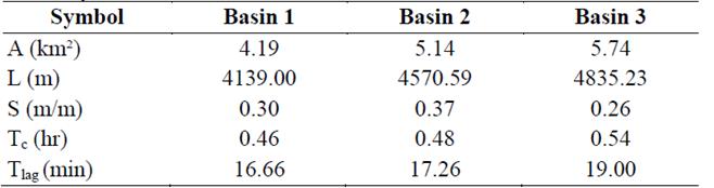
With the aforementioned parameters carried out to calculate the time of concentration and delay of the basin. For the determination of the time of concentration (Tc), there are multiple equations. However, the method that best fit showed was raised by [12], its parameters are disclosed in the eq. (4):
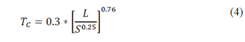
Where L is the distance between the point of study and the hydraulically farthest in meters and S is the average slope of the terrain in the route section (m/m).
Likewise, this parameter is closely linked to the delay time (Tlag), whose calculation was made applying the relation of which Tlag is equal to 0.6×Tc [13].
The previous characteristics and parameters of the basins are summarized in Tables 1 and 2.
5.3. Hydrological model HEC-HMS
With the calculated delay time, the model was created in the HEC-HMS software, in which the area of each of the basins was assigned as input parameters. The method of the curve number of the SCS was established as a method of losses [13] and the Unified Hydrogram of the SCS as rain-runoff transformation method. This hydrograph depends on its definition exclusively on the time of concentration of each one of the basins, the average slope of them and the length of the main channel.
For the election of the curve number (CN) took into account the use of land, the topographic characteristics of the area and the hydrological condition of the basin, which was determined to be good for being protected grazing forests and have a soil covered adequately by vegetable hummus, for which case a representative CN was assumed for the basins of 70. For the case of the basins with grassland cover, taking into account the use of the soil, the characteristics of the area and the hydrological condition of the basin, which for this case was determined to be good because it had a considerable percentage of the area covered with grasses, a representative CN was assumed for all cases of 61.
With the complete HEC-HMS model, the losses of precipitation by runoff and the propagation of the discharges were calculated. However, taking into account that the basins lack instrumentation it was necessary to carry out several iterations with precipitation, for which values of 75, 80, 85, 90, 95 and 100 mm were assumed.
5.4. Hydrological model in Iber
Iber is a hydrodynamic model that allows two-dimensional simulations of different channels. For its implementation, it is necessary to identify the variables required and the considerations to be taken into account when assigning the input data. To start the project it was necessary to define the basin geometry, that was imported from the files generated by the Hec-GeoHMS extension of ArcGIS and to which the respective surface was later created.
The hydrological response of the basin is obtained from the discharges generated by the precipitation assigned in a uniform manner to the model throughout the study area. This is why a specific inlet condition is not defined, but a hietogram is established throughout the basin. On the other hand, the outlet condition and place where the resulting hydrograph will be obtained was established at the lowest point of each basin.
In the definition of the roughness coefficient, it must be borne in mind that this variable is largely dependent on the land use and vegetation coverage of the area. However, bearing in mind that the purpose of this paper is to propose a methodology to calibrate the Manning roughness coefficient through the comparison of the resulting hydrographs of both Iber and HEC-HMS, several modeling was performed for each precipitation, taking "n" values in the range of 0.10 to 0.18 for forest basins, whose definition was based on the value provided by default in Iber of 0.12 for a forest cover. In the case of the basins with grassland cover, the reference value that Iber had by default was taken for a grass or grassland cover of 0.05, adopting a range of 0.01 to 0.05. In some cases, intermediate modeling was carried out or the range was extended to determine with greater precision the value of the roughness coefficient.
The method used to represent the loss in this model corresponds to the one proposed by the SCS [13], in which, under the same criteria established in the HEC-HMS modeling, an NC value of 70 was assigned in the area contributing to the case of the forested basins and an NC of 61 for the basins with grassland cover, while in the main drainage strip a value of 100 was assigned indicating that this entire area is impermeable, that is, that all the water is going to drain.
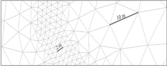
Bearing in mind that the calculations in the IBER models are carried out by applying the resolution of the Saint Venant equations through finite volume schemes in each cell and that the performance of the model will depend on the discretization of the contribution zones; The conception and treatment of each one of the cells through the meshing of the land under study is of great importance [1]. For this reason, an unstructured mesh with two element sizes was built to develop the modeling. In the drainage area, a mesh size of 2 m was assigned, while in the remaining contributing area of each basin size of 10 m was assigned, as shown in the Fig. 1.
Later, using an ASCII format file obtained in ArcGIS from the DEM, the elevations were assigned to the mesh of each of the basins.
6. Results and discussion
Once the modeling was done, in Iber, from the tool calculate> see the information of the process, the results of the calculation of the output discharge and the corresponding simulation time for each basin were obtained. Subsequently, an initial representation of the results was made by means of a hydrogram, where the values of the output discharges obtained from both HEC-HMS and Iber were recorded, discriminating according to precipitation and contrasting the data resulting from the modeling with the different roughness coefficients assigned for both coverages.
Fig. 2 is an example of the water depth map obtained from the Iber post-process. The basin shown is the forest Basin 1.
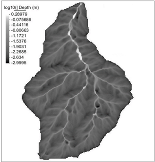
Source: The Authors.
Figure 2. Maps of Maximums, Contour fill of Depth (m), Step 40000. Basin 1 Forests.
6.1. Basins with forest cover
From the simulations carried out for the analysis of watersheds with forest cover, and the comparison made between the hydrograph obtained in the model of HEC-HMS and Iber, it is observed that the limb of the ascent of discharges of the HEC-HMS model shows an earlier response from the basin with a lower rate of increase in discharges. However, when comparing the limbs of the descent of discharges and although they present some similarities, the results of Iber are characterized by presenting a lower rate of decrease, prolonging the hydrological response of the basin for a longer time.
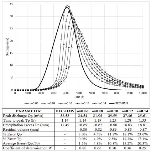
The criterion for selecting the Manning coefficient with the better fit was limited to the variables of peak discharge (Qp) and peak time (Tp) because the distribution of the volumes of the hydrographs from one model to another was very different and not exhibited an appreciable comparison pattern. The Fig. 3 shows the graphics and analytical analysis carried out for the selection of the “n” coefficient.
Source: The Authors.
Figure 3. Comparison of output hydrographs Basin 1 Forests; n=variable; P=75mm; CN=70.
From the graphical analysis, it is observed that the "n" that best represents the peak discharge Qp and the peak time Tp is n = 0.06, analytically corroborated with a percentage error at the peak discharge Qp of 3.0% and 0.0% error at peak time Tp, with an average error of 1.5%. For this case, the coefficient of determination was also the most acceptable. This same analysis was made to each of the modelings of all the basins.
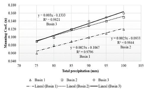
The roughness coefficient obtained from Iber for each basin that best fit the hydrograph of HEC-HMS turned out not to be a single value for a basin since it turned out to be variable in relation to precipitation. Fig. 4 correlates "n" coefficient as a function of precipitation for each basin.
Source: The Authors.
Figure 4. Linear correlation between total precipitation and the Manning coefficient in basins with forest vegetation.
It can be seen that the variability of the roughness coefficient as a function of the total precipitation in each basin can be represented by a linear trend, obtaining coefficients of determination of the order of R²≥0.98. When performing a linear correlation between the Manning coefficient and the peak discharge Qp, an acceptable coefficient of determination is also obtained, this being greater than R²≥0.96 in each basin.
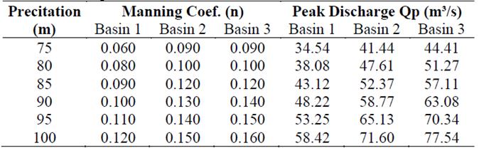
The two previous correlations were constructed based on the results reported in Table 3.
As a result of all the modeling carried out for the calibration of the roughness coefficient of Manning for forests, it was established that the Manning coefficient when estimated based on the hydrogram obtained from the HEC-HMS model is variable depending on the height of the precipitation, obtaining different ranges of variability of the "n" in the different basins for the same precipitation.
Table 3. Resultados de Manning y caudal pico en función de la precipitación para cuencas de bosques.
Source: The Authors.
This variability is associated with the fact that the HEC-HMS model in all precipitation scenarios estimates the response time based on a single lag time "Tlag", so it does not relate the effect of a coefficient variation of Manning in the hydrological response of a basin.
Unlike the HEC-HMS model, the hydrological response in the Iber model is sensitive to the variation of roughness, which affects the distribution of volumes and the response time of the output hydrograph.
6.2. Basins with grassland vegetation
For the grassland vegetation cover, four basins were taken into account, with slopes of the main flow or the longest flow, of 4, 8, 13 and 19%. For these basins, like those of forests, the calibration variables were the peak discharge Qp and the peak time Tp, since there was no close correlation with the volume distribution of the output hydrograph.
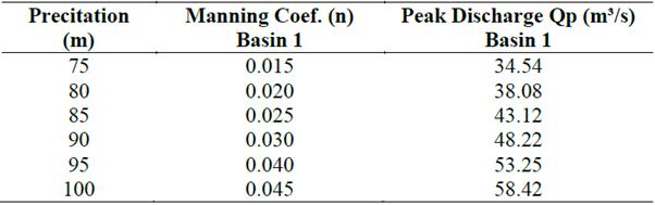
The Basin 1 of Grasslands, with a slope of 19%, once the calibration process was completed presented the results of Table 4.
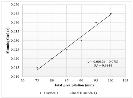
It is appreciated how these results have a linear correlation with a coefficient R²> 0.98 as evidenced in the Fig. 5.
Table 4. Manning results and peak discharge as a function of precipitation for Basin 1 Grassland.
Source: The Authors.
Source: The Authors.
Figure 5. Linear correlation between the Manning coefficient and the peak discharge in Basin 1 with grassland cover.
The behavior obtained in this basin is similar to that obtained for forests, since the parameter that indirectly relates the coverage and land use, is the Curve Number of the SCS, which calculates the abstractions of precipitation and, therefore, determines the effective precipitation (Pe). When having a basin of slope similar to those analyzed in the forest cover, the only variable that would be would be the height of the effective precipitation, which for this case is lower, given that the curve number selected for grasslands was 61 and for forests of 70.
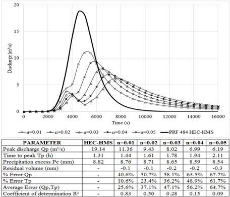
The analysis of the remaining grassland basins showed a considerable variation, as it was observed that the unit hydrograph typical of the SCS was very far from the results obtained from the Iber software. Fig. 6 shows the graphical and analytical analysis obtained for Basin 2 of grasslands with a slope of 8% and with total precipitation of 75 mm.
Source: The Authors.
Figure 6. Comparison of output hydrographs Basin 2 Grasslands; n=variable; P=75mm; CN=61; PRF 484 HEC-HMS.
It should be noted that the results of the Iber model are totally far from the output hydrograph, with an average error of peak discharge Qp and peak time Tp greater than 30%, making a calibration attempt with the hydrograph typical of the SCS unfeasible. Also, it is pertinent to highlight the fact that not even the Iber model with a Manning of 0.01 (typical coefficient of very smooth surfaces such as glass, plastic or copper [14]) manages to assimilate the behavior obtained from the HEC-HMS.
As a consequence of the previous result, it was necessary to use a unit type hydrograph of the SCS that will better represent the conditions for land with a low slope. Table 5 shows the other adaptations that the hydrograph of the SCS has; From this table, it can be seen that there are hydrographs for rural basins with slight to very flat slopes, which can simulate with a better adjustment the conditions of the basins with grassland cover.
Table 5. Hydrograph peaking factors and recession limb ratios
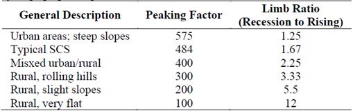
Source: Unit Hydrograph (UHG) Technical Manual. National Weather Service - Office of Hydrology Hydrologic Research Laboratory.
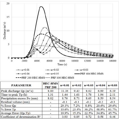
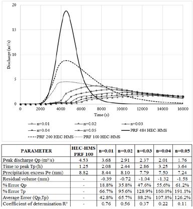
Including the hydrographs for basins with slight slopes (PRF = 200) and very flat slopes (PRF = 100), the following analyzes are obtained for the same previous case of Basin 2 of grasslands with a 75 mm precipitation (Fig. 7). And the same for Basin 4 of grassland, which is the basin of the study with the lowest slope (S = 4%) (Fig. 8).
Source: The Authors.
Figure 7. Comparison of output hydrographs Basin 2 Grasslands; n=variable; P=75mm; CN=61; Various PRF HEC-HMS.
Source: TheAuthors.
Figure 8. Comparison of output hydrographs Basin 4 Grasslands; n=variable; P=75mm; CN=61; Various PRF HEC-HMS.
The visualization of the output hydrographs of all the basins was cut to a shorter time, with the sole purpose of being able to correctly appreciate the graphs.
The previous analysis was carried out for each of the basins, varying the precipitation from 75 to 100 mm, without obtaining any correlation between the typical hydrograph of the SCS (PRF 484), nor with the hydrographs of the SCS for rural basins with slight slopes (PRF 200) to very flat (PRF 100).
The calibration process for basins with grassland vegetation coverage was not possible for basins with medium to low slopes, because the hydrograms obtained with the Iber model when compared with the typical unit hydrograph of the simulated SCS using the HEC-HMS software had no correlation whatsoever.
Using other type hydrographs of the SCS method for rural basins with slight to very flat slopes, there was a better approach in the distribution and response behavior of the hydrograph; However, the results continued to be uneven, so the process was terminated by the methodology initially proposed for the calibration of both forest and grassland cover.
In order to make a check of the distributed hydrological model to detect any error or inconsistency in which it could have been incurred, a variation was made in the wet-dry limit between 0.001 to 0.0001 m, under the conditions of permeability and in the size of the cells. By making these variations to the models, it was possible to appreciate that the lower the slope of the basin, the more alterations were observed in the hydrological response due to the modification of these parameters.
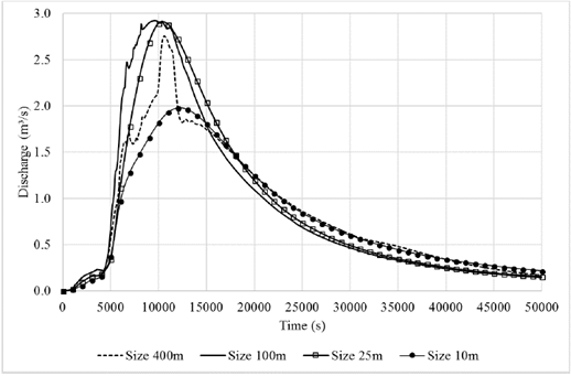
Fig. 9 shows the fluctuations that the model of the Basin 4 of grasslands presents with large cell size, a situation that was evident in the other basins, but it could be seen how this phenomenon was accentuated since it is the basin with the slope flatter. For this sensitivity analysis, the basins were established as impervious with effective precipitation of 10 mm. This same analysis was carried out in the other basins.
From the same sensitivity analysis, it can be seen that the size of the mesh has a significant effect on the output hydrograph, noting important differences, especially in the magnitude of the peak discharge and the time to the peak, the difference is more noticeable in conditions of low precipitation and in basins with flat slopes.
Source: The Authors.
Figure 9. Comparison of output hydrographs with the cell size variation. Basin 4 Grassland; Impervious; P=10mm.
Based on all the previous analyses, it can be deduced that the hydrological response of basins with low slopes in the Iber model is more sensitive to the variation of the construction parameters of the model (wet-dry limit and mesh size), impacting in a significant in the output hydrograph, appreciably varying peak discharge and peak time.
It was also possible to observe how the intensity of the rain plays a fundamental role and, therefore, not negligible in the estimation of the hydrological response for flat basins, making the inclusion of this variable indispensable in the methods of calculating the time of concentration and lag time.
To conclude the analysis, it is concluded that, in the analysis of basins with grassland cover with low slopes, a correlation between the Iber model and the HEC-HMS model was not achieved. In these basins, the intensity of precipitation and the Manning coefficient have a relevant effect on the behavior of the output or response hydrograph of the basin, since the comparison model is not sensitive to the variation of these variables.
7. Conclusions
For each one of the basins selected for the analysis, which are seven in total, where there are three for forest cover and four for grassland cover, the response hydrograph for several precipitation intervals with a duration of one hour was determined, using the HEC-HMS software. These hydrographs were the starting point to start the calibration process, which consisted of an iterative process, where several simulations were carried out in the Iber model, taking as a variable to determine the "n" of Manning, until obtaining the hydrograph that best will be adjusted to that obtained from HEC-HMS.
From the analysis of the calibration process for the forest vegetation cover, it was observed that the hydrographs obtained in Iber had a different volume distribution to those of HEC-HMS, where the limb of the ascent of discharges of the HEC-HMS model shows a response earlier in the basin with a lower rate of increase in discharges. However, when comparing the limbs of the descent of discharges and although they present some similarities, the results of Iber are characterized by presenting a lower rate of decrease, prolonging the hydrological response of the basin for a longer time. Consequently, the objective parameters to select the "n" coefficient with better fit were summarized in the peak discharge (Qp) and peak time (Tp).
It can be concluded that, the roughness coefficients obtained for each forest basin after the calibration stage are not a single value, but that a range of variation was obtained as a function of precipitation, preventing the determination of a value or an approximate range for each type of coverage, since even the ranges obtained from a basin compared with another basin of the same type of coverage are inconsistent. Such limitation is associated with the fact that the HEC-HMS model uses a single parameter to determine the response time of the basin, which is the lag time (Tlag) which, in turn, is a function of the concentration-time (Tc) and does not consider the alteration caused in the response times due to the variation of rainfall intensity.
In the analysis of the calibration process for the basins with grassland cover, it was possible to demonstrate that there was no close correlation for basins with medium to low slopes with the typical hydrograph of the SCS (PRF = 484) and although others were resorted to unit type hydrographs for basins with slight to very flat slopes of the SCS, there was no approach in the distribution and response of the hydrograph.
From the calibration of the basins with grasslands and forests, it can be inferred that, under the methodology proposed for this project, it is not possible to perform an adequate calibration for the basins where the average slope of the channel or flow line farthest are medium to low ; It is important to clarify that the only difference in the calibration process between forest and grassland cover ends up being the effective precipitation Pe, which is a function of the assigned CN curve number, which indirectly associates the use and coverage of the basin. In this project, it was identified as a characteristic that the forested basins had considerable slopes, unlike the basins covered with grasslands, where the average and low slopes predominated.
It was possible to demonstrate how the hydrological response in flat basins in the Iber model is more sensitive than with the basins of medium to high slope, before the variation of the construction parameters of the model; as they are mesh size and wet dry limit.
Finally, it was determined that the hydrological response and the volume distribution in the hydrograph obtained with Iber are sensitive to the variation of rain intensity and the roughness coefficient of Manning, these variables being more determinant in the flat basins.

