


 Inglês (pdf)
 Artigo em XML
 Referências do artigo
 Enviar este artigo por email
 Citado por SciELO
  Citado por Google
  Similares em
SciELO
Similares em
SciELO  Similares em Google
 Permalink
1. Introduction
A type of geometric entities very common in computer vision, in physics, medicine and in general in nature are those caused by intercepting a plane with a cone [1-3,27]. The interception of these generates a type of curves that in geometry are called conical. Depending on the cut these are classified as parabola, ellipse, circumference, hyperbola and degraded conic [4].
The mathematical model that describes the behaviour of a conic obeys a quadratic equation with an independent variable and uniform parameters. A thematic that arises in the application of the conics to different physical problems, consists in determining the parameters of the quadratic equation given a set of coordinates in rectangular plane. To solve this, in the literature different approaches and methodologies have been proposed, which can be classified into three large groups. First, we have the methods based on geometric distance where the purpose is to minimize a cost function given a constraint; usually the cost function and constraint are associated with the parameters of the conic. Secondly, we have the approaches based on parametric models and Euclidean distance, where the purpose is to solve an unrestricted optimization problem by means of an iterative method in this category can also be classified the methods based on the Hough transform (HT) [25], and third, probabilistic methods where a probability distribution function is assumed on parameters and data [5,6].
Naturally, each approach has characteristics of the proposed model. As an example, the methods based on probabilistic models are highly robust to noise, as well as to atypical information; however, they have a high cost of computation [6]. On the other hand, the algorithms based on Euclidean distance are relatively simple to implement, unfortunately they present drawbacks with data with a high level of curvature. On third place, methods based on geometric distance usually have optimal local solution, although they are sensitive to noise, occlusion and atypical information present in the data [7]. Therefore, the application of a particular approach depends on the nature of the data.
The detection of ellipses using HT has been introduced since the last two decades due to the robustness to occlusion, although the most common variants of HT (standard HT, probabilistic HT, combinatorial HT, geometric symmetry) are not suitable for locating ellipses [25], there are modifications of the HT that seek to solve this problem, such as fast ellipses HT, random HT, Hybrid HT, which compute good results but present some restrictions such as sensitivity to disconnected pixels, projective distortion, besides, these only detect ellipses and circles due to their application in digital images [26].
The methods based on geometric distance with non-convex restriction on the parameters ignore the discriminant of the quadratic equation to infer the parameters of an ellipse or hyperbola, because the conditions of Karush Kuhn Tucker (KKT) establish that to compute the global minimum in this case is not a guarantee, but it allows to compute a local minimum or saddle point [7-9].
The methods taught in the state of the art generally convert the nature of the discriminant into an equality as a restriction, in this manner the solution is computed by means of the Lagrange function where the optimal solution is found by means of the generalized eigenvectors of the covariance matrix [7,10]. Similar models are detailed in [11,12,27]. However, these remain bound to a convex function as a restriction, restricting the solution to a particular case.
In this article a method that uses the discriminant of the quadratic function to suggest using the Tikhonov regularization model to estimate the parameters of a hyperbola or ellipse (Tikhonov L-Curve Conic Fitting (TLCCF)) is proposed. On the other hand, the procedure introduces an instrument that allows to automatically determine the optimal value of the regularization parameter that maximizes the curvature of L-Curve, that is, a search is performed on the entire solution space without simplifying the nature of the restriction function; in this manner a strategy that emerges from the traditional solution, which is linked to the eigenvectors associated with the design matrix of the model is explored. The obtained results show that the method is robust against significant noise variations because the method regularizes the solution without ignoring the dynamics of the discriminant of the quadratic equation. On the other hand, an application of the method for the detection of conics present in a digital scene (image) is introduced as an exploratory mode. The main contributions of the article submitted are the following:
Documentation of a methodology that allows to infer the parameters of a conic given real observations, which is robust to the noise present in the data.
Report of the evaluation of the methodology against different methods proposed in the state of the art.
This article consists of two sections, which are described below:
On section two the methodology is introduced, describing each of the stages that conform it, as well as the mathematical development of the model and its solution.
On section three the experiments are described along with the results debating the cons, the benefits; as well as the future works that must be addressed. Lastly the research conclusions.
2. Methodology
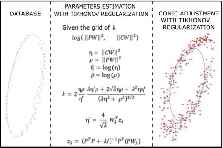
The working methodology consists of adapting the Tikhonov regularization method for the paradigm of tuning the parameters of a conic given a set of coordinates in the two-dimensional plane. The test procedure considers noise both in a real context (digital image scene) and synthetic (simulated data contaminated with noise), the construction of the method considers three sequential stages. In the first place, a database constituted with ellipses and synthetic hyperboles is made from a structure used in the literature used for this purpose [10]. Secondly, it solves a restricted and regularized optimization process that computes the parameters of the conic given a set of correspondences on the rectangular plane; finally, in the fourth stage a validation process of the methodology is performed, in this it is determined the confidence of the method for different noise levels making a comparison with two classic methods documented in the state of the art. Fig. 1 shows a block diagram summarizing the methodology.
Experiment
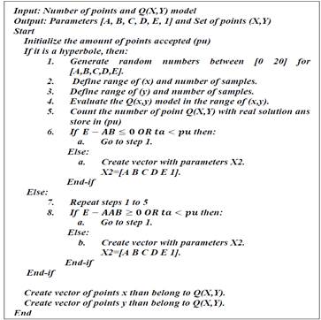
In this stage an algorithm is built for the generation of points (x,y) belonging to a conic with the purpose of generating different inputs for the Montecarlo analysis and thus evaluate the behaviour of the algorithm under different cases. The generation of synthetic conics is achieved through an algorithm that allows the random generation of ellipses and hyperboles using the discriminant of the quadratic equation. In this way, each rectangular coordinate belonging to the synthetic conic is contaminated with different levels of Gaussian noise.
The design of the algorithm takes into account as input variables the number of minimum coordinates with which we want to work and the option to generate an ellipse or a hyperbola. The flow diagram of this algorithm is shown in the algorithm 1.
The rectangular coordinates are contaminated with white noise, with distribution N (0, σ), where the value of σ depends on the signal to noise ratio.
regularization
Considering the least squares problem, the idea is to find the minimum distance solution of the eq. (1)

where ϑ is the design matrix, b is a known solution vector and x is the unknown. The problem described above is badly conditioned; therefore, it is resorted to impose such a restriction.

Where λ is known as the regularization parameter and the amount ∁(x) the restriction. When ∁(x)= ||Lx||2 is used, the above problem is called Tikhonov regularization [23]. i.e.:
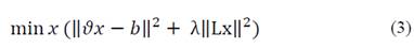
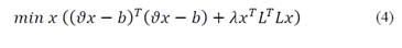
If b=0, the above formulation takes the following form:
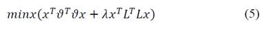
The formulation can be used to estimate the parameters of a conic. Firstly, the conic Q (x,y) is defined quadratically as shown in eq. (6).
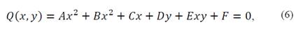
This is a convex entity where the parameters W T = [A,B,C,D,E,F] describe and define the conic’s nature.
This can be expressed in matrix form as shown in eq. (7).
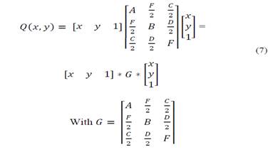
Now the idea is to formulate a restricted optimization problem to compute the parameters W of the conic, given a set of correspondences in the rectangular plane, this is:
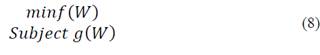
Which is equivalent to:
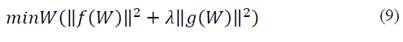
f(W) is the cost function and is given by the following equation:

Eq. (10) is equivalent to the first term of the eq. (5), where P is the design matrix containing the information of the rectangular coordinates to which the conic belongs, and n is the total set of correspondences in the rectangular plane. Finally, g(w) is given by the eq. (11).
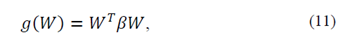
with ( given by the following expression:
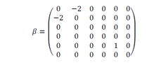
The value of the matrix ( is inferred like this, if we define the point ∆ as the cut point of the conic 𝑄(𝑥,𝑦) with a straight line at infinity, it can be shown that if:
Δ>0 the conic 𝑄(𝑥,𝑦) is a hyperbola.
Δ=0 the conic 𝑄(𝑥,𝑦) is a parabola.
Δ<0 the conic 𝑄(𝑥,𝑦) is an ellipse.
We proceed to define two points at infinity 𝑃1 𝑇=[𝑥′𝑦′0] y 𝑃2 𝑇=[𝑥 𝑦 0], therefore the parameter Δ can be written like this
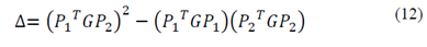
Operating we get the following:
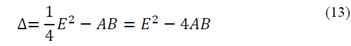
Which is known in the literature as a discriminant of the conic, note that this is independent from the point at infinity selected and follows a non-homogeneous behaviour (in the case of the ellipse and hyperbole), it also only depends on the parameters of the conic: additionally for the case of an ellipse and hyperbole the behaviour of Δ is not convex [7] Note further that the value Δ can be written in a matrix form like this:
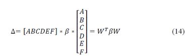
Which obeys to the restriction of the optimization problem posed previously on the eq. (9). In this manner, performing the comparison with the problem of Tikhonov regularization we have in this case that the term 𝜗x=𝑃W, b= 0 and finally
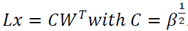 Thus, the Tikhonov problem takes the following form (eq. (15)) for the tuning of the parameters of a conic.
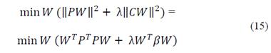
The problem posed in the eq. (15) can be partially solved (global minimum is not guaranteed) in the event that an elliptical or hyperbolic conical body is present [24]. For this it is differentiated in relation to W the target function like this:
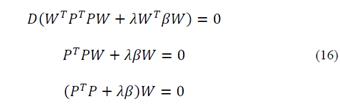
Commonly, from the eq. (16) the eigenvalue of the matrix is inferred 𝑃𝑇𝑃 (covariance matrix) that allows it to be defined as positive, this value corresponds to the value Of λ, thus 𝑊 will be the eigenvector associated with it, however the above is only valid in the case where 𝑔(𝑊)=1 [7], therefore this solution will be omitted because it belongs to a particular case. Now the term α = 𝑃𝑇𝑃 +λ( is defined, therefore the problem of inferring the parameters 𝑊 is summarized in solving the following linear problem (eq. (17)).
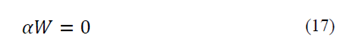
Where the trivial solution W =0 it is not of interest, this suggests that it is necessary to re-edit the value of the parameters, for this purpose we make use of the homogeneity of the second order equation of the conic which allows to normalize the parameters, this is with ||W|| =1 Therefore, the problem takes the following form (eq. (18)).

The above problem can be solved by performing decomposition in singular values to the matrix α, meaning, α =USV T . It can be shown that the solution to the problem described above is given by the last column of the matrix V T , for more detail of this procedure the reader can consult [20].
It is noteworthy that the final solution is based on the set of rectangular coordinates of the conical body, the constraint and the regularization parameter being this unknown.
using the L - Curve method
The formulation described in the previous section presents the difficulty of not automatically computing the value of λ. To do this, we suggest to apply the concept of L-Curve, which is a tool that allows to graphically represent the Tikhonov model (eq. (19)) given the regularization parameter. The purpose is to perform a simulation of the L-Curve for different values of λ, these represent possible solutions to the estimation problem, the method ends up solving an optimization problem that allows to infer the optimal value of λ.

The representation in the two-dimensional plane of the final correspondence vector is known in the literature as the L-Curve, in which the value of the regularization parameter is implicit. The selection of this should guarantee a corner as defined as possible in the L-Curve, i.e. the idea is to compute the value of λ which is located at the corner of the L-Curve. The reasoning behind this choice is that the corner separates the flat and vertical parts of the curve where the solution is dominated by regularization errors and disturbance errors, respectively. Hansen and O'Leary introduced calculating this value as the coordinate in the two-dimensional plane that maximizes the curvature of the L-Curve [21].
Now the criterion for selecting the optimal value of the regularization parameter corresponds in computing the value λ that maximizes the curvature k of the L-curve. First, the following terms are defined:
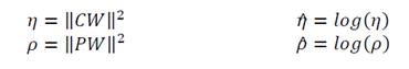
It can be shown that the curvature k is given by the following equation [21]
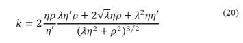
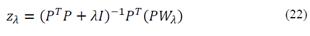
Where η is the first derivative of η in regards to λ. It can be demonstrated that η is given by the following:
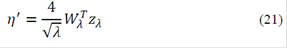
With
2.4. Validation of the methodology
In this stage, the performance of the proposed estimation method is validated. Therefore, the method is evaluated from two approaches, one of classification and the other of estimation. In the first approach the Monte Carlo method is used for the random generation of conics and thus calculate the average success rate, when evaluating ∆. In the second approach, Gaussian white noise is added to the conics generated in the experiment and the average RMS error is calculated. In the classification experiment, different conics are simulated based on the algorithm 2, performing 100 iterations of Monte Carlo for 7 different noise levels, which allows obtaining 600 iterations in the experiment. The range of noise variation is [0 25]% of SNR - (Signal to Noise Ratio).
In order to quantify the performance of the proposed methodology, two state-of-the-art methods were selected to estimate the parameters of the conic and perform a performance comparison of the estimation approaches, performing the tests proposed in this stage. The first method suggested is the Least Squares (LSF) [22], which aims to estimate parameters looking for the minimum error between the data and the proposed model without any restriction. The second approach is a regularization method with homogeneous restriction (LSFC) where the restriction function is convex, in addition the validation tests are implemented in the conic 2𝑋2+𝑋2+2.8284XY−2=0, which is the input of tests in some similar works [7,9,10].
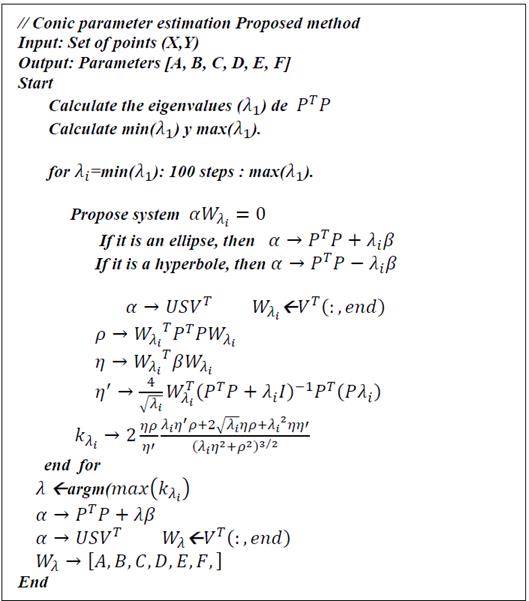
3. Analysis and results
In this section we present the results obtained by tuning the parameters of a conic from the distribution of rectangular coordinates of interest contaminated with noise in a synthetic scenario and a case study with a possible application of the method. In this stage it is possible to show that the TLCCF method allows to infer the intrinsic parameters of a conic, as shown in Algorithm 2 Wλ =[ABCDEF] The presentation of the results is divided into two sections, firstly, the problem of correctly classifying the nature of the conic using the random conic generation algorithm is evaluated, i.e., the purpose is to determine if the method is in the capacity to discriminate the nature of the conical body (hyperbole, ellipse). Secondly, the estimation problem is considered by calculating the RMS error between the estimated value and the real value, then a comparison is performed between the different methods under study and observations are performed based on the results. It is important to highlight that the parabolas are not considered in this work, because an entity with these characteristics can’t present variations with noise because it will immediately become an ellipse, therefore, the experiments do not apply to this conic, additionally in this case the problem is simplified because the constraint for this entity presents a convex behaviour which is the optimal analytical solution.
Tikhonov regularization
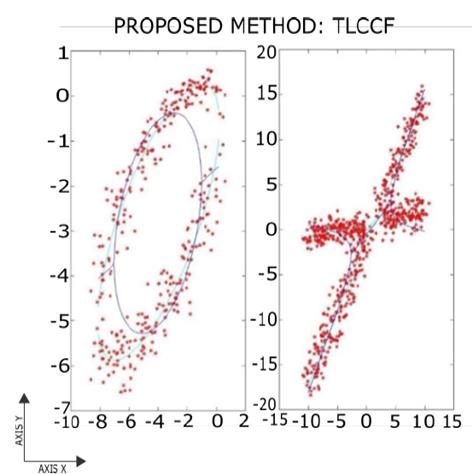
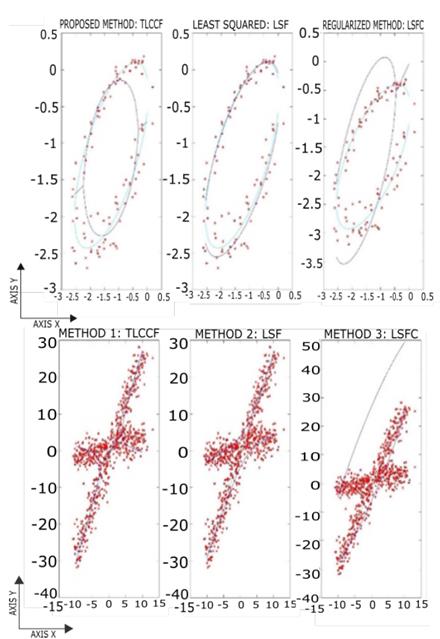
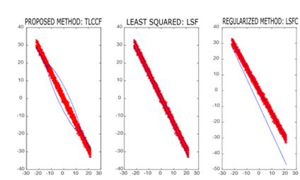
For the different figures that will be presented in this section, the aquamarine blue data refers to those with no noise and the king blue data represents the performance of the proposed method. In Fig. 2 the estimation result applying the TLCCF method to an ellipse and hyperbola contaminated with Gaussian noise SNR of 15% is shown. It can be verified that the results of the method under study are similar to the ideal model considering the noise present in the data. This allows to deduce that the regularization captures the non-linear nature of the data and the noise does not produce a considerable deviation in the estimation.
In Fig. 3 the estimation results for the three methods evaluated with a SNR of 15 are observed. From this it can be noted that the three methodologies guarantee the estimation of an ellipse; however, the LSFC method presents an error greater than that of the other methodologies. At low noise levels (SNR = 15) the LSF method demonstrates to have the smallest error when approaching the ideal model. In the case of hyperbole, the behaviour is maintained; however, it is emphasized that the LSFC option does not guarantee the estimation of a hyperbola failing the classification test.
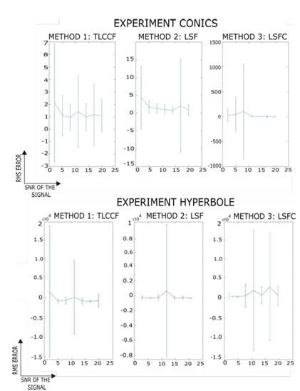
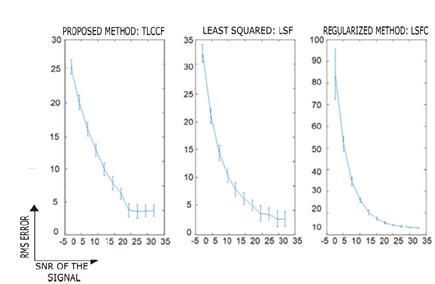
In order to not only describe the results qualitatively, the results of the Monte Carlo experiment are shown to evaluate the performance of the method. In the first part of the experiment, the number of correct answers produced by the estimation is calculated, and in the second part of the experiment, the RMS error is calculated between the estimated and ideal model. For the 200 conics, the SNR level of the noise is varied with values of SNR = [20 17 14 11 8 5 2], where the quantities close to zero mean that the noise ratio is much higher than the signal, which implies considerable noise levels. This experiment is applied to all methodologies and their performances are compared. In Fig. 4 you can see the average RMS error and its deviation for the three proposed methodologies in the Monte Carlo experiment. To evaluate performance, the magnitude of error and a minimum deviation of the data will be sought.
From this Fig. 4. It can be shown that the TLCCF proposal presents the best performance for the highest noise levels, which for the purposes of the graph are the SNR values close to zero. This guarantees a better performance with the presence of atypical data. On the other hand, LSF and LSFC present better performances with low noise levels this can be seen in Fig. 4 where these methods show a lower deviation and average error regarding TLCCF.
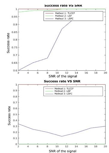
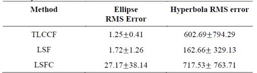
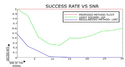
When calculating the RMS error in the different noise levels it is observed that LSF shows a better performance in comparison to the other methodologies obtaining an error value equal to 164.38. These results are shown in Table 1. Although these results suggest that LSF tends to generate a smaller error, this approach does not necessarily guarantee the restriction of the adjustment, which can cause a conic with a different nature to the real one to be estimated. Therefore, the RMS value should not be the only measure of performance and the success percentage should be observed. In Fig. 5, the percentage of success for the Monte Carlo experiment is shown with values of SNR = [20 17 14 11 8 5 2].
Source: The Authors.
Figure 5. Percentage result of success for different SRN, left ellipses and right hyperboles.
In this scenario, the TLCCF proposal has a 100% accuracy efficiency for the adjustment of conics, this means that the method guarantees an estimation with restriction, unlike the other methodologies where performance decreases with increasing noise deviation. This factor is of vital importance to evaluate the methodology, because it is a priority to guarantee the type of conic to avoid an erroneous tuning in the parameters and thus its respective nature.
In order to make a direct comparison with other works of the state of the art, the same set of tests for the conic 2𝑋2+𝑋2+2.8284𝑋Y−2=0, which corresponds to an ellipse, was carried out. In Fig. 6 we can observe the results of estimation for each of the three proposed methods for a Monte Carlo experiment, in this example it is observed that TLCCF does not guarantee the best error; however, it adjusts the conic to guarantee that it is an ellipse. On the other hand, note how in Fig. 7 the TLCCF method guarantees the restriction of the model despite increasing the noise present in the data and Fig. 8 shows that the TLCCF method has the lowest RMS error for considerable noise variations.
Source: The Authors.
Figure 6. Estimation result for the three methods under study with the conic [7].
Although the RMS error plays an important role in measuring the quality of an estimation a minimum error does not guarantee a correct estimation. This is largely due to the fact that the presence of atypical data can strongly deviate the estimation and, for purposes of this work, change the nature of the conic.
Images
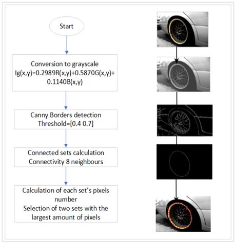
In this stage a possible practical application of the TLCCF method is presented, it should be noted that its evaluation is exploratory, since the purpose of this test is to demonstrate the versatility of the proposed method and not the exhaustive evaluation in a real case. The chosen application is the detection of the parameters of a conical object given its contour. To achieve this application, a classical segmentation method is used in digital image processing [15,17-19], as described in Fig. 9.
In the state of the art there are different databases for the detection of patterns using images where they focus on the capture of different objects, people, textures, urban designs, among others [13], however, a database with the capture of conical objects in a scene is not reported; for this reason, a collection of 100 images that meet the conditions of the proposed application is made and thus evaluate the behaviour of the methodology in different contexts [14].
In Fig. 10 the result obtained by applying the detection method and the TLCCF setting for an image given the contour is shown. This shows the correct functioning for the proposed problem because the estimation manages to adjust to the conical profile of the object despite the atypical information present in the data.
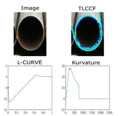
Note also how the method computes the regularization parameter that maximizes the curvature near the origin of the L-Curve.
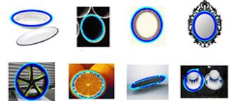
In Fig. 11 the result of the proposed methodology for different objects is summarized. It is clarified that, in the database, the images only contain objects with elliptical contour, because in the real world it is common to find this type of morphologies, however, hyperbolic figures are difficult to capture in a real case. Therefore, hyperboles are not considered.
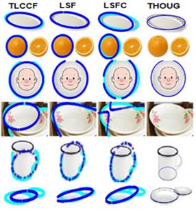
Finally, Fig. 12 shows the results for six images in the database. In all three cases, TLCCF performs a better adjustment than the other methods. This performance is mainly due to the fact that the proposed methodology is robust to the presence of occlusion in the data, which is not present in the other methodologies where the presence of overlap generates erroneous estimations, reaching an incorrect conical determination. This is important because it corroborates the robustness of the method when there is atypical information, which was evidenced in the results obtained with synthetic data.
Source: The Authors.
Figure 12. Estimation result for the three methods under study with images from the database [7].
Fig. 12 expose the results when testing 4 methods of contours estimation. From these, their accuracy can be compared and conclude that the Houge transformed for ellipses (THOUG) [26] is quite accurate to estimate the contour of images even though this is partially hidden, while for those containing noise in the scene, the adjustment is not precise and, in many cases, it can’t be carried out.
4. Conclusions
A methodology was presented that allows to compute the parameters of a conic given a set of rectangular coordinates by means of a Tikhonov regularization model, which once it is resolved is automatically tuned by means of the L-Curve technique. Based on the results, high robustness of the TLCCF is shown given considerable levels of noise and partial occlusions present in the data: although LSF computes good results for moderate levels of noise, there is no guarantee to determinate the real nature of the conic under study, because it is a model without restriction, contrary to the TLCCF that allows in all cases to estimate with the real nature of the quadratic function. The above is very important because it is desirable that the model captures the real tendency of the data to later be replicated in a real situation.
In the case of the problem explored, it is important to highlight that the method of parameters estimation depends on the data provided for its training, for this reason the selection of an adequate segmentation method of points of interest is of vital importance. Although the methodology presents a high robustness under the appearance of atypical data, data with high deviation from its real value can lead to erroneous adjustments or an adjustment with incomplete information, leading to estimate a conic with a high effective RMS error. For this reason, it is important to direct efforts in the design of a method that allows the conic's contour segmentation minimizing the probability of choosing edges belonging to other entities.

