


 Inglês (pdf)
 Artigo em XML
 Referências do artigo
 Enviar este artigo por email
 Citado por SciELO
  Citado por Google
  Similares em
SciELO
Similares em
SciELO  Similares em Google
 Permalink
1. Introduction
Solar energy is one of the main renewable energy resources that has been used increasingly during the last 10 years, because of its advantages, such as being pollution-free and noiseless [1]. However, electric faults in PV arrays generate significant power losses, which is why researchers are looking for effective ways to detect and classify these faults in order to improve system reliability and efficiency [3].
The performance of a photovoltaic system mainly depends on the temperature of operation of the solar panels, solar radiation and the presence of faults that may cause significant power losses. Monitoring systems for photovoltaic arrays represents a high cost of investment for the owners. This is why in small photovoltaic arrays, like residential applications, users do not regularly check for faults, leading to losses in energy and safety [2]. This research proposes a characterization method by only measuring the voltage and current at the output of the array to obtain the VP curves without using multiple voltage and current sensors in each string, leading to a low-cost solution capable of detecting and classifying electric faults in PV array systems.
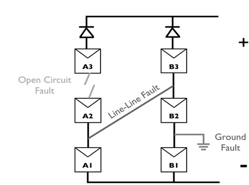
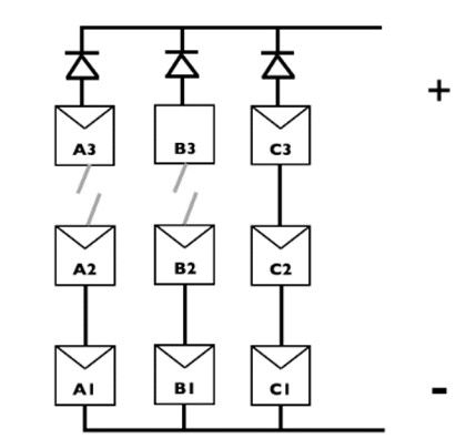
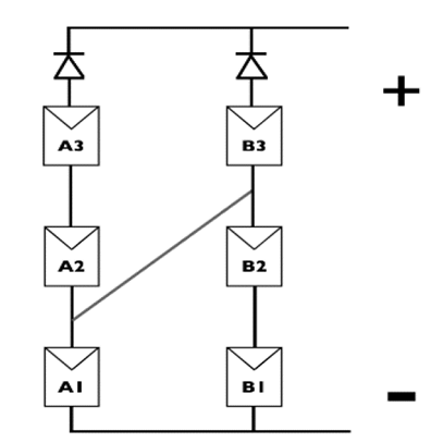
Fig. 1 shows a circuit diagram of the three main faults that are analyzed in this work. The line-to-line fault is causing low impedance between two different strings in the PV array. The open circuit fault is generating a faulty string, disabling the power delivery corresponding to that string because the current in the string is zero. The ground fault is causing low impedance between a node of a string and the negative wire conductor.
A ground fault in a PV array produces a low impedance path between a Current Carrying Conductor (CCC) and the ground/earth [4]. To detect ground faults, PV systems usually use devices such as Ground Fault Detection and Interruption Devices (GFDI), Residual Current Monitoring Devices (RCM), and Insulation Monitoring Devices (IMD). These ground fault detection devices have some limitations because they are based on differential current measurement methods, which may create blind spots during low solar radiation, night, cloudy days or partial shading [4,5].
A line-to-line fault can reverse the current flow through the faulty string. The amplitude of the fault current depends on the voltage difference between the points of the strings that are causing the fault [4]. Over Current Protection Devices (OCPD) are used to detect line-to-line faults, but these devices have some limitations if the current is lower than a threshold [4,5].
An open circuit fault occurs when a solar panel is disconnected, making the current of all the solar panels associated to the same string zero. In this case, supposing that the solar radiation in each solar panel is the same, the voltage at the output of the array will not be affected. Only the current will be reduced (subtracting the current that is not being supplied by the faulty string), leading to a loss of power.
To prevent significant power losses and reduce the negative economic and safety impacts, it is important to detect the existence of electric faults in PV array systems on time. Conventional fault detection and protection methods like GFDI, RCM, IMD and OCPD are not able to detect faults on time due to different solar radiation conditions.
Researchers have developed multiple techniques to detect electric faults in PV array systems. Recent reviews of proposed techniques are reported in [4,6,7]. In [8,9], authors developed Time Domain Reflectometry (TDR) techniques for PV fault detection and localization. The proposed method has limitations because the installation circumstances can easily change the parameters of the system. Therefore, it is important to measure the characteristics of the signal response just after installing the PV system. In [10-13], the authors propose voltage and current measurement methods to detect faults in a PV array system. The methods were able to increase the accuracy of the failure judgement but need multiple voltage and current sensors, one per each string of the PV array.
Intelligent systems have been proposed to detect faults in PV systems. Neural networks were employed in [14,15] as pattern recognition systems. Non-supervised learning was employed in [16]. Extreme machine learning was proposed in [17] and fuzzy systems in [18]. All these methods require large amounts of data about the system’s operation under normal conditions to train the pattern recognition systems.
Fault diagnosis analyses from different types of systems, such as hydroelectric generators, were reviewed as referents to identify algorithms and methods that could be applied in photovoltaic array systems. In [19], a neuro-fuzzy algorithm was proposed to detect faults in hydroelectric generators. In [20-22], fault diagnosis systems were proposed to detect mechanical problems in the rotor by using different spectral estimation techniques, based on SVM (Support Vector Machine) and PCA (Principal Component Analysis).
Therefore, none of the previous works has presented a characterization of electric faults in PV arrays by only measuring the VP (Voltage and Power) curve at the output of an array without using multiple voltage and current sensors in each string.
This research uses the one-diode solar cell model to represent the functional behavior of photovoltaic array systems under different fault, temperature and solar radiation conditions, in order to make a characterization of the VP curves at the output of the photovoltaic array. The results from this work can open the possibility of designing and developing low-cost solutions capable of detecting faults in photovoltaic array systems.
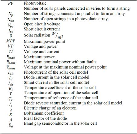
This article is divided as follows: Section 2 presents an electric model of a photovoltaic module in order to simulate faults in photovoltaic array systems. Section 3 presents a characterization of the VP curves under different fault conditions. Section 4 presents the results and conclusions. Table 1 shows the nomenclature used in this article.
2. Photovoltaic array electric model
Solar panels are composed of multiple solar cells connected in series. A photovoltaic array can be made by connecting multiple solar panels. In this section, a one diode solar cell model is described in order to simulate photovoltaic arrays of dimensions N s X N p which means the array is composed of N p strings connected in parallel, and each string is composed of N s solar panels connected in series.
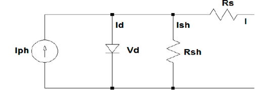
Fig. 2 shows an equivalent circuit of a one diode solar cell model based on [12].
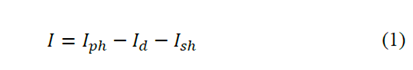
The output current I can be described with the following equation:
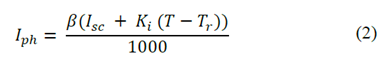
The photocurrent I ph can be described with the following equation:
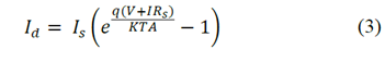
The diode current I d can be described with the following equation:
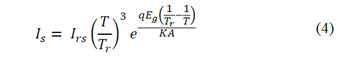
The diode reverse saturation current I s can be described with the following equation:
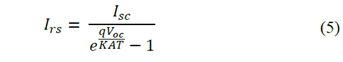
The diode reverse saturation current at the reference temperature I rs can be described with the following equation:
The shunt current I rs can be described with the following equation:
With this model, the VI (Voltage and Current) curve at the output of the solar cell can be obtained by defining solar radiation and the solar cell’s temperature of operation. The model of a photovoltaic array can be represented by multiplying the voltage and current by the number of solar cells connected in series and in parallel, respectively.
A. Experimental validation of the electric model using one solar panel
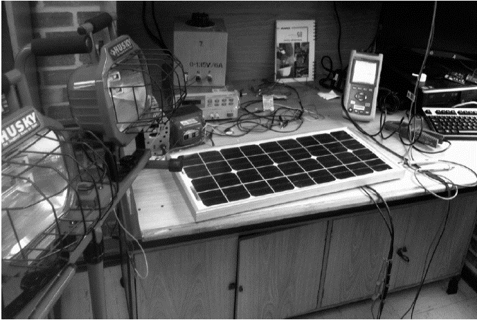
The first step of this research was to experimentally validate the electric model of a solar cell. To do this, the VI curve at the output of a 20W solar panel with Voc = 21.6V and Isc = 1.31A was measured. The 20W solar panel was connected to a variable load to obtain the VI curve by measuring the voltage and current with a power analyzer, FLUKE 43B, and a digital multimeter, FLUKE 8010A. Two 600W HUSKY lamps were used to simulate different solar radiation levels, and radiation was measured with an LT300 luxometer. The electric model was validated using Matlab and Simulink, comparing the VI curve obtained experimentally to the VI curve generated by the model.
Fig. 3 shows a photo of the 20W solar panel used in the lab to measure the VI curve in order to validate the electric model.
B. Experimental validation of the electric model under different fault conditions
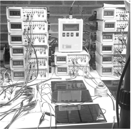
After validating the electric model with the 20W solar module, another experiment was performed using six 2W solar panels to build a 3x2 PV array. The array’s VP curve was measured under different fault conditions in order to validate the model. Fig. 4 shows a photo of the 3x2 PV array under different fault conditions. In this experiment, the voltage and current of each solar panel were measured simultaneously with a digital multimeter, FLUKE 8010A. Solar radiation [W/m2] was measured using a pyranometer, and the simulation of solar radiation was generated using two 600W HUSKY lamps. Different VP curves were obtained according to each type of fault with these measurements.
Source: The Authors.
Figure 4. Photo of the 3x2 PV array used to validate the electric model under different fault conditions.
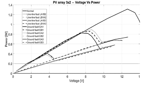
Fig. 5 shows the VP curves of the three types of faults that were obtained experimentally in the 3x2 PV array. An array with the same topology was built in Simulink/Matlab to simulate the operation under the same fault conditions to validate the solar cell model. The electric model of a 3x2 PV array under different fault conditions was validated with this analysis.
Source: The Authors.
Figure 5. Experimental VP curves of a 3x2 PV array under line-to-line faults and ground faults.
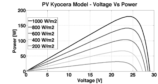
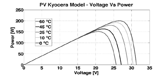
The electric model was also validated by simulating the VP curve of a 170W Kyocera PV module under different temperature and solar radiation conditions. The output power of a solar panel is proportional to the solar radiation and inversely proportional to the temperature of operation. Fig. 6 and Fig. 7a present the VP curves of a 170 W Kyocera PV module under different levels of solar radiation and temperature of operation.
Source: The Authors.
Figure 6. VP curves of a 170W Kyocera PV module under different solar radiation levels.
Source: The Authors.
Figure 7a. VP curves of a 170W Kyocera PV module under different temperatures of operation
Fig. 6 shows that the power at the MPP (Maximum Power Point) at the output of a PV module changes for different levels of solar radiation, while the voltage remains almost constant.
Fig. 7a shows that, for different levels of temperature, the power and voltage at the MPP at the output of a PV module changes.
3. Characterization method
After validating the PV array model in Section 2 under different fault conditions, different array configurations between 2x2 and 7x7 PV with blocking diodes were simulated in order to characterize the different VP curves that can be obtained at the output of each array depending on the type of fault and the dimensions of the array.
A. Open circuit faults
Open circuit faults are symmetrical between strings. In an open circuit fault, the voltage at the output of each string is the same, assuming that all the solar panels have the same technical specifications and that all of them are under the same solar radiation and temperature conditions. This means that if a string has an open circuit fault, the voltage at the output of the remaining strings will still be the same. This is why the voltage at the maximum power point in a VP curve will be the same even if the array changes its number of strings - because, by adding or removing strings, the equivalent circuit is only changing the output current of the full array.
Fig. 7 b shows an example of a 3x3 PV array with an open circuit fault in the first (left position) and the second (middle position) string. These two faults generate an open circuit in the two strings, only making the power that is produced from the third string available. In this example, the power at the output of the array will be the third part of the power of the full array without faults.
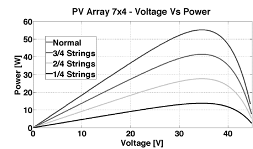
Fig. 8 shows a simulation of all the possible VP curves that can be obtained in a 7x4 PV array model under open circuit faults with a constant solar radiation of 1000 W/m2. The curve labeled as ‘normal’ represents the operation of the array without faults. The curve labeled as ‘3/4 Strings’ represents an open circuit fault in one of the four strings of the array. The curve labeled as ‘2/4 Strings’ represents an open circuit fault in two of the four strings of the array. The curve labeled as ‘1/4 Strings’ represents an open circuit fault in three of the four strings of the array.
Fig. 8 shows that the voltage at the MPP of the array VP curve is the same when the system has an open circuit fault. The VP curves of the array under open circuit faults have the same voltage at the MPP (35V), which is the same voltage of the MPP of the curve that represents normal operating conditions (without faults). This means that the output power at the MPP of the array can be described as:
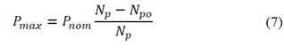
Where,
P max is the maximum power of the VP curve, P nom is the maximum nominal power of the VP curve (without faults), N p is the number of strings in the array, and N po is the number of open strings in the array.
From Eq. (7) the number of strings that are opened in a PV array can be calculated as follows:
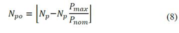
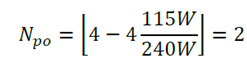
For example, by using Eq. (8) in a 3x4 array system with a nominal power of 240W for a given solar radiation (12 solar panels of 20W each). If an MPP measurement shows that the power is 115W, it means there are two faulty strings (rounding to the lower and nearest integer):
B. Line-to-line faults
Line-to-line faults in PV array systems are symmetrical between strings. Fig. 9 shows a 3x2 PV array under a line-to-line fault between solar panel A1 and B2, called LA1B2 here. In the line-to-line fault presented in Fig. 9, the voltage at the output of PV module A1 will be the same as the sum of voltages at the output of PV modules B1 and B2, generating a current between the two strings and disabling the power output from PV module B3.
The line-to-line fault LA1B2 is symmetrical to a line-to-line fault LA2B1. LA1B3 fault is symmetrical to LA3B1, and LA2B3 is symmetrical to LA3B2. In the same way, in a 3x3 PV array, LA1B2 is symmetrical to a LA1C2. Therefore, because line-to-line faults are symmetrical, the number of different line-to-line faults that can be differentiated is equal to ( N s −1).
Fig. 10 shows the VP curves at the output of a 7x4 PV array with different line-to-line faults.
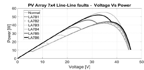
Fig. 10 shows that a line-to-line fault generates two peaks in the VP curve. The first peak (lower voltage peak) occurs at different voltages, depending on the line-to-line fault, while the second peak has a small variation when faults occur. The voltage at the first peak for each faulty condition is approximately 5V (LA7B1), 12V (LA7B2), 17V (LA7B3), 24V (LA7B4), 28V (LA7B5) and 33V (LA7B6). Meanwhile, the voltage at the second peak (higher voltage peak) of each curve is between 36V and 38V.
From the previous analysis, we can conclude that a VP curve with two peaks is a characteristic of a line-to-line fault. Thus, by measuring the position of the first peak, it could be possible to detect and classify this kind of electric fault in a PV system.
B. Ground faults
Ground faults are symmetrical between strings. Fig. 11 shows a 3x2 PV array under a ground fault in solar panel B2, which is called GB2.
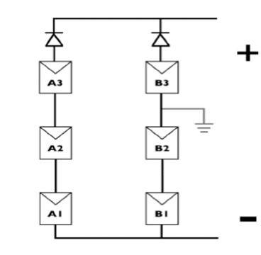
Note that ground fault GB1 is symmetrical to ground fault GA1. Fault GB2 is symmetrical to GA2, and GB3 is symmetrical to GA3.
Fig. 12 shows the VP curves at the output of a 7x4 PV array with different ground faults. It shows that a ground fault has the characteristic of generating two peaks in the VP curve as line-to-line faults. And again, the voltage at the first peak serves as an indicator of the position of the ground fault in a PV array.
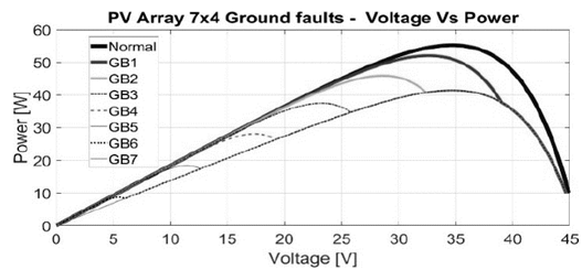
By comparing the VP curves from Figs. 10 and 12, we can conclude that both types of faults (line-to-line faults and ground faults) generate a similar behavior in the VP curves.
This means that the following equivalents are:
LA1B2 = GB1 (1 PV of difference)
LA1B3 = GB2 (2 PV of difference)
LA1B4 = GB3 (3 PV of difference)
LA1B5 = GB4 (4 PV of difference)
LA1B6 = GB5 (5 PV of difference)
LA1B7 = GB6 (6 PV of difference)
4. Analysis of the VP curves under faults
In the characterization of line-to-line faults, the positions of the two peaks, P1 (lower voltage peak) and P2 (higher voltage peak), were analyzed in terms of percentage variations of voltage and power with respect to the point of reference, which is the MPP of the VP curve without faults. A trend curve was obtained depending on the type of line-to-line fault and the dimensions N s X N p of the array.
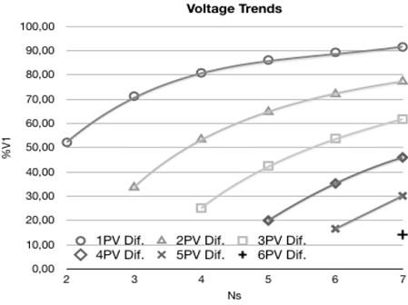
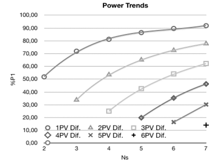
Fig. 13 shows the percentage variation of voltage in peak P1 depending on the number of solar panels connected in series (Ns) in the array and the number of PV’s of difference in a line-to-line fault.
Source: The Authors.
Figure 13. Voltage at peak P1 for line-to-line faults from 1PV to 6PV of difference.
Fig. 14 shows the percentage variation of power at peak P1 depending on the number of solar panels connected in series (Ns) in the array and the number of PV’s of difference in a line-to-line fault.
Source: The Authors.
Figure 14. Power at peak P1 for line-to-line faults from 1PV to 6PV of difference.
From Figs. 13 and 14, it is possible to obtain a first estimate of the position of peak P1 by considering the number of solar panels connected in series. In order to improve the estimate of peak P1’s position, a second trend curve was used, which considered the number of strings connected in parallel in order to obtain a voltage compensation level.
The voltage compensation level in this work refers to a percentage of voltage associated to Np that can be added to the percentage of voltage associated to Ns in order to obtain a more accurate voltage level of peak P1.
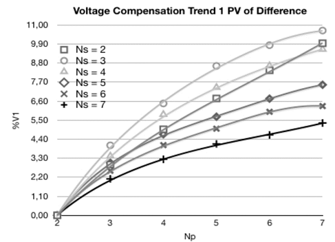
Fig. 15 shows the voltage compensation at peak P1 for line-to-line faults with 1 PV of difference. It is possible to obtain a more accurate voltage level of peak P1 by adding the voltage compensation to the voltage that is obtained from the trend curves from Fig. 13, taking into account dimensions Ns and Np of the PV array.
Source: The Authors.
Figure 15. Voltage compensation at peak P1 for line-to-line faults with 1PV of difference.
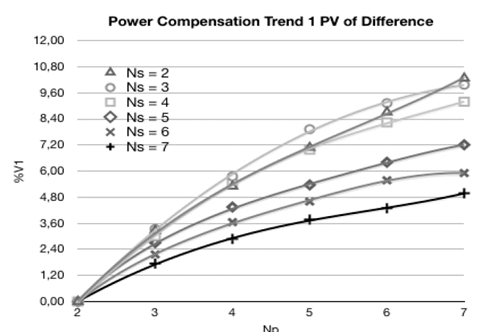
Fig. 16 shows the power compensation at peak P1 for line-to-line faults with 1 PV of difference. It is possible to obtain a good estimate of the power at peak P1 by adding the power compensation to the power that is obtained from the trend curves that are in Fig. 14, taking into account dimensions Ns and Np of the array.
Source: The Authors.
Figure 16. Power compensation at peak P1 for line-to-line faults with 1PV of difference.
It is possible to obtain a good estimate of the position of peak P1 when a line-to-line fault occurs by using the trend curves from Figs. 13, 14, 15 and 16.
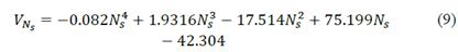
Eq. (9) represents the percentage variation of voltage at peak P1 for line-to-line faults of 1 PV of difference according to the parameter Ns.
Eq. (10) represents the percentage variation of power of peak P1 for a line-to-line fault of 1 PV of difference according to the parameter Ns.
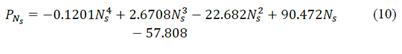
For the particular case of a 4x3 PV array (Ns = 4), by using eq. (9, 10), the percentage of voltage and power at peak P1 is VNS= 80.9% and PNS 81.35%.
Eq. (11, 12) represent the percentage variation of voltage and power at peak P1 for a line-to-line fault of 1PV of difference depending on the parameter Np for the particular case of a PV array with Ns = 4.


For a 4x3 PV array, by using eq. (11, 12) the percentage of voltage and power at peak P1 is VNp = 3.4% and PNp = 3.1%.
Now, by using equations (9- 12) it is possible to estimate the voltage of the first peak P1 by using the following equation:
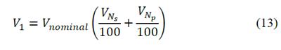
Where V1 is the voltage at the peak P1, V nominal is the voltage at the MPP without faults, V Ns is the percentage variation of voltage of peak P1 compared to the voltage at MPP associated with N s , V Np is the percentage variation of voltage at MPP associated with N p . By using eq. (13), the voltage at peak P1 can be calculated:

This means that the voltage at peak P1 when a line-to-line fault with 1 PV of difference occurs in a 4x3 PV array will be at 84.3% of the nominal voltage of the array at the MPP when there are no faults.
Fig. 17 shows a simulation of different VP curves for a 4x3 PV array with different types of line-to-line faults. The curves represent the operation of the array with line-to-line fault LA1B2, which is a fault of 1 PV of difference, line-to-line fault LA1B3, which is a fault of 2 PV of difference, and line-to-line fault LA1B4, which is a fault of 3 PV of difference.
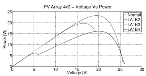
The MPP of the VP curve without faults is (19.54V, 23.29W). From the curve that represents the line-to-line fault LA1B2, the voltage of peak P1 is 16.46V and corresponds to 84.24% of the nominal voltage. By applying equation 13 for a line-to-line fault of 1 PV of difference, the estimated voltage of peak P1 is 16.48V (84.3% of the nominal voltage), which is a very good estimate to obtain the position of peak P1. The same operation can be performed using the power equation trends to estimate the power at point P1.
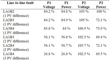
Finally, all the VP curve trends were calculated between 2x2 and 7x7 PV arrays for line-to line faults between 1 and 6 PV of difference to obtain the characterization of the faults and be able to calculate the position of the first peak according to the dimensions of the PV array. Table 2 shows the voltage and power levels corresponding to peak P1 and peak P2 in a 4x3 PV array under different line-to-line faults.
Table 2. Voltage and power levels in peak P1 and peak P2 in a 4x3 PV under line-to-line faults.
Source: The Authors.
It is possible to estimate if an open circuit fault occurs when there is only one peak in the VP curve by knowing the nominal VP curve at the output of a PV array system, and then by applying the equations mentioned before. When there are two peaks in the VP curve, it is possible to estimate the position of peak P1 to identify the type of line-to-line fault that is presented in the array. All this can be done with minimal instrumentation, by only measuring voltage and the current at the output of the array to obtain the VP curve.
In a future work, designing an algorithm capable of classifying different types of faults could be possible by measuring the temperature and solar radiation in a PV array system. This can be done by applying the results presented in this work after knowing the temperature and solar radiation levels during the system’s operation in order to estimate the nominal VP curve at the output of the array without faults.
5. Conclusions
Electric faults in PV arrays can generate a local and global maximum point in the VP curve at the output of the array. A simulation of multiple PV array topologies from 2x2 to 7x7 under different electric faults was performed in order to get the local and global maximum power point position from the VP curve at the output of the arrays. A characterization of the VP curves at the output of different photovoltaic array topologies under line-to-line faults, open circuit faults and ground faults was presented based on the location of the local and global points on the VP curve at the output of an array. The characterization of electric faults was validated experimentally by measuring the VP curves at the output of multiple PV array topologies.
Ground faults at the last PV of a string generate the same VP curve of an open circuit fault with one faulty string. Line-to-line faults produce an equivalent circuit similar to ground faults, producing the same VP curves, so they cannot be differentiated easily. By applying this characterization method, and by only measuring the voltage and the current at the output of an array to get the VP curve, it was possible to identify and estimate the position of the local and global points in the VP curve according to each type of fault for multiple PV array topologies.
In a future work, the characterization method can be implemented inside an algorithm to detect and classify these three faults in a photovoltaic array system by only measuring the voltage and the current at the output of a photovoltaic array to obtain the VP curve, significantly reducing the number of sensors needed to diagnose the system. In order to design an algorithm based on the characterization method, it is important to measure the temperature of the PV modules, solar radiation and the VP curve at the output of an array fast enough (<1s) to prevent significant solar radiation variations.

