


 Inglês (pdf)
 Artigo em XML
 Referências do artigo
 Enviar este artigo por email
 Citado por SciELO
  Citado por Google
  Similares em
SciELO
Similares em
SciELO  Similares em Google
 Permalink
1. Introduction
The pollutants discharged into semi-enclosed bays are mixed with the receiving water through physical processes such as convection transport and dilution diffusion [1]. In the process of exchanging water between the inner and outer bays, the concentration of contaminants gradually decreases, which improves water quality. The exchange and mixing processes are closely related to self-purification capacity and the transport of nutrients, among other factors, which has aroused the interest of researchers, increasingly frequently in studies of water quality in estuaries and coastal areas [1-6]. As a concept related to water exchange, transport time scales such as water age, flushing time, residence time and renewal time are often used as parameters to represent the time scale of physical transport processes [1]. These time scales can describe how some water quality parameters (e.g. eutrophication) change under different conditions [1,7]. The exchange of water in a bay is the result of the complex interaction of factors such as geographical features, waves, tides, winds and currents, and therefore knowledge of the scale of transport time is of great importance for protecting the marine environment and maintaining the ecological balance of coastal areas [1]. Residence time has marked effects on the ecological quality of water bodies in semi-enclosed bays and estuaries [8]. In semi-enclosed domains such as Buenaventura Bay the water renewal capacity is mainly controlled by the exchange flow between the outer and inner domains as well as by the inner circulation [8]. Internal circulation is affected by bathymetry, among other aspects. This parameter plays a very important role in the vulnerability of water bodies to eutrophication and pollution [9]
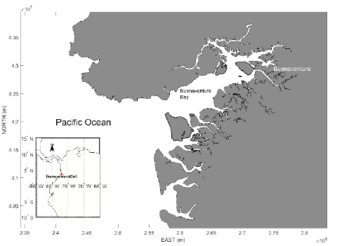
In Buenaventura Bay (Fig. 1), Colombia's main port terminal on the Pacific Ocean operates. It is located between latitudes 3° 44' and 3° 56' N and longitudes 77° 1' and 77° 20' W. It is 21 km long and its width varies between 3.4 km at the sea exit and 5.5 km in the internal part. It is narrow and elongated, follows an orientation SO to NE with an approximate extension of 682 km2 and average depths of 5 m. has a single entrance known as La Bocana, formed by a strait of 1.6 km [10]. Its interior is an estuarine system due to the combination of the salty water of the Pacific Ocean with the fresh water of the rivers and estuaries that flow into it, such as Dagua (66 m3/s), Achicayá (99 m3/s), Humane (30 m3/s), Gamboa (30 m3/s), Aguacate (10 m3/s), San Antonio (20 m3/s), Hondo (10 m3/s) and Agua Dulce (80 m3/s). The values of tributaries discharges were obtain from [11]. The external sector has direct communication with the open sea and receives all its influence [10].
In order to improve competitiveness, the port terminals carry out dredging activities of their access channel that seek to take it to a final depth of 17.7 m in the inner part of the bay where the city of Buenaventura is also located, officially declared by the Congress of the Republic of Colombia as a Special, Industrial, Port, Biodiverse and Ecotourism District in 2013. Through this port, Colombia exports 80% of its coffee and 8.7% of all its international maritime trade.
To study the change in residence time in Buenaventura Bay due to the dredging process, a combination of a two-dimensional hydrodynamic model and a particle trajectory model was used.
2. Implementation of the model
A two-dimensional finite element model RMA2 [12] was used to provide the values of the water surface elevation and the components of the horizontal velocity vector. It computes water surface elevations and horizontal velocity components for subcritical, free-surface flow in two-dimensional flow fields [13]. The RMA2 model is frequently used in physical oceanography to represent processes such as tides and currents in coastal regions and estuaries, its use has been documented by [14-21]. RMA2 solves the depth-averaged equations of fluid mass and momentum conservation in two horizontal directions. These equations can be written as follows:
Momentum in X-direction equation:
Y-direction momentum equation:
Continuity equation:
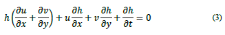
where, h is depth, u, v are velocities in the Cartesian directions, ρ is density of fluid, E is eddy viscosity coefficient, g is acceleration due to gravity, n is Manning’s roughness, δ is empirical wind shear coefficient, v α is wind speed, φ is wind direction, ω is rate of earth’s angular rotation and 𝜙 is local latitude.
The Lagrange trajectory model used determines the movement of discrete particles from an Euler field of velocities provided by the RMA2 model, for which the following difference equation is solved.
Where, x,i are the values of the particle position at time t, y u,i corresponds to the velocity field. This equation is solved numerically using the Runge-Kutta method of fourth order, to minimize error [8]. The particles were virtually released two days after the RMA2 model was initiated to avoid initial instability due to their starting or heating period and their trajectory was determined until the end of the hydrodynamic simulations.
2.1. Definition of the domain and computational mesh
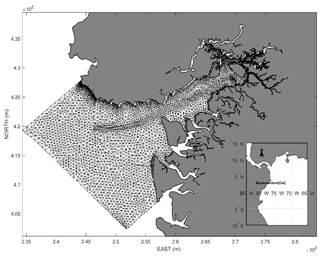
The finite element mesh developed for Buenaventura Bay is shown in Fig. 2, where the internal and external part of the mesh is represented with triangular elements of different sizes. The finite element technique allows the irregular geometry of the coastline to be captured more accurately and ensures increased resolution in areas of special interest. 19,672 elements with dimensions between 500 and 15 meters and 43,604 knots were used.
2.2. Boundary and initial conditions
For the simulations with forced astronomical tides and considering that direct measurements of sea levels in open waters are not available, tidal conditions were used provided by the harmonic constituents extracted from the tide gauge station located in the inner part of the Buenaventura Bay, that has hourly data since 1953. The T-Tide software [22] was used to extract the main tidal harmonics. 68 tidal harmonic constituents with a significance level of 95 % were extracted. In models of relatively small and semi-enclosed bays, the forcing of tides in open boundaries are more important than other forcing ones such as local winds [23]. This was confirmed by the sensitivity analysis, for which the model showed no response to variations in the magnitude and direction of the wind, and finally for this condition constant data of 1.5 m/s of wind in the Northwest direction were used.
It was necessary to specify the initial conditions for elevation of water levels and velocity throughout the domain. These were supplied by a previous 24-hour run for the same domain, which in turn was initialized at zero values for water level elevation and velocities at all mesh knots. The model was fed with the discharges from the Dagua, Achicayá, Humane, Gamboa, Aguacate, San Antonio, Hondo and Agua Dulce tributary rivers and estuaries.
2.3. Calibration and validation
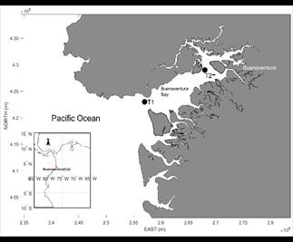
For the calibration and validation process of the hydrodynamic model, data from measurements of water levels (tide) and currents with AANDERA equipment taken between August and September 2017 during the study of the master plan for the sewage system of the District of Buenaventura were used. To determine the direction and magnitude of the currents, a continuous recording RCM9 LW was used. Measurements were made at 15-minute intervals. Water levels were also measured with a WLR7 tide gauge. The location of the measuring stations used in the calibration and validation process is shown in Fig. 3. The measurement equipment was alternated in these stations in two field campaigns, Table 1 shows the dates during which the equipment was deployed and the purpose of the data collected in them. The Manning coefficient was varied in the range from 0.05 to 0.035 m1/3/s, while a constant value was used for the Eddy viscosity coefficient of 10 m2/s, the values of both coefficients were obtained in the calibration process by error assay.
2.4. Evaluation of the model
The measurement of accuracy from statistical techniques is very common among researchers to quantify the performance of hydrodynamic models [24]. The techniques used in this study are detailed below.
2.4.1. Correlation coefficient
The correlation coefficient (R) is a common indicator of whether two sets of measured data and predicted are related. The correlation coefficient R measures the trend of predicted and measured (observed) values in a linear variation. This statistic can vary in the range of [-1.1], negative values indicate that measured and predicted data tend to vary inversely. R does not show how significant the correlation is, as it does not consider the distribution of measured and modeled data. That is, even if the correlation is close to 1, the predicted and observed values may not coincide with each other; they only tend to vary in a similar way. The formula for the calculation of R is presented in eq. (4) [24]:
With Xm the set of measured values and Xc the set of calculated values; σm and σc are the standard deviations of measurements and predictions respectively, < > denote average.
2.4.2. SKILL - concordance index
The Concordance Index, or skill, represents the relationship of the Mean Square Error and the Potential Error as shown in eq [5]. The index range is between zero (no correlation) and 1 (perfect fit ) [20].
Xm be a set of N observed and measured values, and Xc be a set of N calculated and predicted model values. X̅ is the average of the modeled or measured variables. The use of this statistic has some disadvantages; relatively high values (more than 0.65) of "Skill" can be obtained even for poor model fit, which leaves a narrow range for calibration, therefore, this should be used along with other statistical techniques to judge the accuracy of the prediction [24].
2.4.3. RMS - quadratic mean error
RMS is a commonly used measure of the size of discrepancies between the values predicted by a model and the values actually measured (observed) [24].
The ranges of reference values considered for the evaluation of the model results with respect to these parameters are shown in Table 2.
Table 2 Range of acceptable statistical measurement techniques based on the literature.
| Ref. | Water level | Actual speed | ||||
| RMS - % Maximum variation | Correlation coefficient | Skill | RMS - % Maximum variation | Correlation coefficient | Skill | |
| [25] | 7.8-8.9 | 0.96-0.97 | - | 8.6-10 | 0.91-0.93 | - |
| [26] | 3.5-9.3 | 0.97-0.98 | - | 10.1-22.2 | 0.63-0.9 | - |
| [27] | 2 - 6.5 | - | - | - | - | - |
| [28] | - | - | - | 3 12 | - | 0.74-0.99 |
| [29] | - | - | 0.97 -0.99 | - | - | 0.68-0.9 |
Source: Adapted from [24]
2.5 Simulation scenarios
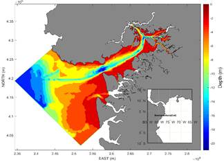
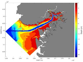
Two simulation scenarios were used to determine the effects of dredging on hydrodynamic conditions in Buenaventura Bay. The first corresponded to the initial bathymetry with the depth of the seabed before the dredging interventions (Fig. 4). The coastline and the bathymetric points for the simulation domain in the coastal area of Buenaventura Bay were obtained from the nautical charts of the Dirección General Marítima (DIMAR) available for the study area, using charts COL154 and COL155 with official bathymetric information available and updated to 2017. For the second scenario, the bathymetry of the access channel at depths of 17.7 m in the inner part of the bay and 18.7 m outside the bay was adjusted and idealized over the domain (Fig. 5). The two scenarios were compared with runs of the hydrodynamic model where the only variation was bathymetry.
Source: The Authors
Figure 5 Bathymetry scenario two, with modified access channel to dredging depths
In this study we used a particle trajectory model to estimate the effects of dredging on the time of residence inside Buenaventura Bay. The average residence time is the time needed for a percentage of a conservative substance to leave the bay [30]. Authors such as [30] recommend a percentage of 67%. A total of 100 particles distributed to the interior of Buenaventura Bay were virtually released, the residence time representing the period required for each particle to leave the Bay from each release point. To determine the effects of dredging on the bay's retention time, a one-year simulation was performed using the 2D model previously calibrated and validated with both scenarios. The effects on residence time were assumed by the differences in the two simulation scenarios.
3. Results and discussion
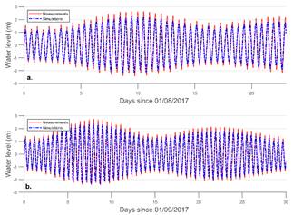
The bottom roughness was the main calibration parameter of the hydrodynamic model proposed for Buenaventura Bay. The RMA2 model allows assigning discrete bottom roughness values to different areas of the simulation domain, for this specific case 7 Manning coefficient values were applied to the same number of element types. The types of elements were differentiated by depth, proximity to open borders and to the coast. The maximum variation of the RMS for both calibration and validation with water level data was between 9.4 and 10.7 % while the correlation coefficient was higher than 0.96 and the minimum predictive ability was 0.94. These values are adjusted in the range suggested by [24]. The graphical comparison between the measured data and the results of the hydrodynamic model for the tide are presented in Table 3 and Fig. 6, where the fit between the time series can be seen confirming what was shown by the statistical valuation techniques.
Table 3 Evaluation techniques of the hydrodynamic model.
| Reference | Water level | Actual speed | |||||
|---|---|---|---|---|---|---|---|
| RMS - % Maximum variation | Correlation coefficient | Skill | RMS - % Maximum variation | Correlation coefficient | Skill | ||
| T1 (WRL7) | 9.4 | 0.975 | 0.97 | - | - | ||
| T2(RCM9) | - | 10.5 | 0.94 | 0.89- | |||
| T1 (RCM9) | - | - | 12.3- | 0.84- | 0.81 | ||
| T2(WRL7) | 10.7 | 0.961 | 0.94 | ||||
Source: The Authors
Source: The Authors
Figure 6 Time series comparison of measured and simulated water levels with RMA2. a). Monitoring station 1 (T1). b). Monitoring station 2 (T2).
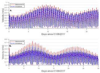
The comparison of the velocity data showed, as did the water levels, that the model reproduces the measurements appropriately, both in calibration and validation, as can be seen in Fig. 7. The statistical values used in the model evaluation revealed that the values obtained (see Table 3) are in the acceptability ranges suggested by [2].
Source: The Authors
Figure 7 Comparison of time series measured and simulated velocity values with RMA2. a). Monitoring station 1 (T1). b). Monitoring station 2 (T2).
According to the values of the parameters RMS, Correlation Coefficient and Skill presented in Table 3 for both water levels and current velocities, the authors considered the model calibrated and validated.
The results of the model showed a good approach with the field measurements, however, in the specific case of the tide a very good fit was achieved during the ebb tide reflux, while during the flow the peaks were not captured perfectly. This situation may suggest that the flow dominates the hydrodynamic regime of Buenaventura Bay, however there are few previous studies that allow us to conclude on the matter. The results of the current velocities showed an equal tendency to reproduce the peaks of the water levels with a smaller approach. Some simplifications made at the time of implementation of the model, among them, attributing constant flows to the main tributaries and neglecting the smaller tributaries can influence the peaks of water levels and transport during ebb and flow, this simplification is due to the scarcity of data measuring the flows of these streams. Despite this, the statistics used to evaluate the accuracy of the model yielded values with acceptable error ranges.
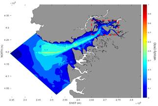
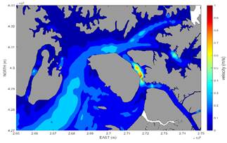
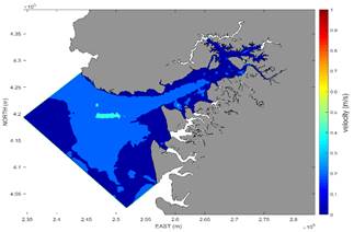
From the results of the calibrated and validated model, the spatial distribution of the mean velocity (m/s) in Buenaventura Bay is presented in Fig. 8 for the scenario with bathymetry before the dredging intervention. The highest proportion of the domain has average speeds of less than 0.30 m/s. In the sectors close to the access channel, the model showed average speeds between 0.3 and 0.6 m/s. Few areas in the bay have speeds close to 1 m/s or higher, see box in the discontinuous red line in Fig. 8, enlarged in Fig. 9; according to the results of the extended period run (simulation of a year) the only area where speeds of the order of 1 m/s are recorded corresponds to a strait formed between the island and the mainland of Buenaventura (see Fig. 9).
Source: The Authors
Figure 8 Average speed scenario I, without dredging. Area in red rectangle corresponds to zoom Fig. 9
The application of the particle trajectory model in the velocity fields of the initial bathymetry scenario without dredging shows that the spatial distribution of residence time varies from 1.3 to 89 days (Fig. 10). In the outer part of the bay the lowest residence times are presented, generally less than 30 days, these zones correspond to a more direct communication with the Pacific Ocean and in general show higher average speeds compared to the internal part of the bay. In the middle part of the bay, residence times of between 30 and 60 days are obtained.
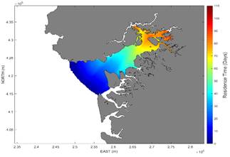
Source: The Authors
Figure 10 Residence time Buenaventura Bay Scenario I, initial bathymetry without dredging
By varying the bathymetry of the access channel in the way projected by the dredging works (scenario 2), lower velocities are obtained than those of scenario 1. In Fig. 11 it can be appreciated how the spatial variation of the velocity fields decreases significantly in comparison with scenario 1 shown in Fig. 8. This local decrease in the velocity field implies an increase in residence time which was confirmed by the results of the particle trajectory model applied to scenario 2 (see Fig. 12).
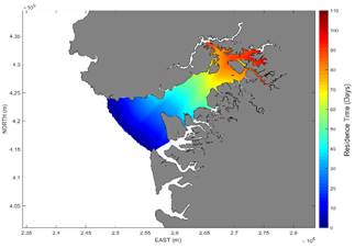
Source: The Authors
Figure 12 Residence time Buenaventura Bay Scenario II, final bathymetry, with dredging
When making the difference with the results of the particle trajectory model, it was found that the deepening of the access channel of Buenaventura Bay can increase the residence time in the same by up to 12 days depending on the area of the same, as shown in Fig. 13.
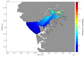
Source: The Authors.
Figure 13 Increase in residence time in days in Buenaventura Bay due to the effect of dredging the access channel.
A complete and rigorous simulation of residence time requires a greater availability of freshwater input data, which in turn can have a marked seasonality in the amount of flow, given the periods of winter and summer: in the rainy season the rivers drastically increase their flows and therefore their discharge to the bay. For the development of this work it was not possible to count with the time series of the tributary rivers flows, for this reason their discharges were considered constant throughout the simulations. The flows of the rivers during the rainy season can influence the decrease of the time of residence in the bay in relation to the increase of flows.
These aspects were not considered in this work and therefore corresponds to one of the simplifications made in the implementation of the model.
Later on, it is necessary to consider the influence of the of tributaries discharges in order to make a more precise estimation of the time of residence of the bay. Since the hydrodynamic model reproduces the velocity fields very well, the results obtained in estimating the residence times are considered close to the behavior of this parameter in the bay. New considerations must be made including tributary discharges and thermohaline conditions. The estimation of the time of residence was considered with the average and constant discharge of the tributaries, the results obtained are indicators of average conditions in the bay of Buenaventura. The extreme values due to seasonal changes generated by the maximum and minimum flows and by the time series of the tributaries discharges were not considered in this study.
The Residence time identifies the time it takes for a particle to leave the study domain. The results of the simulations show that the time of residence in Buenaventura Bay has a high spatial variation, from a few days at the exit of the bay, where it communicates with the Pacific Ocean, to several months in the innermost part. This variation is related to currents, given that in the area where there is a shorter residence time, in addition to coinciding with a more direct communication with external waters, there are current velocities of greater magnitude. The higher currents force the plots of water to leave the bay faster.
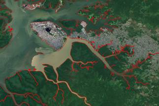
The high residence times of the bay of Buenaventura suggest that it functions as a trap for the sedimentary solids discharged by the tributary rivers. The high load of solids thrown by the tributary rivers (Fig. 14) and the high residence time combined with weak currents cause the solids to sediment and as they accumulate in the bed of the bay, they generate greater requirements for dredging over time.
4. Conclusions
Buenaventura bays has high residence times which negatively affects the possibility of self-purification of the sheet of water. The pollutants and nutrients discharged into this body of water tend to be concentrated because of the low dilution potential shown by the high residence times found.
Higher residence times in Buenaventura Bay are related to the magnitudes of weak currents in most of it, in general there are magnitudes lower than 0.4 m/s in a large portion of it, as a consequence the water remains a longer time.
The dredging processes produce a local decrease in the velocity fields inside the Buenaventura Bay, generating a drastic increase in residence time. This increase can be up to 12 days in some places.

