


 Inglês (pdf)
 Artigo em XML
 Referências do artigo
 Enviar este artigo por email
 Citado por SciELO
  Citado por Google
  Similares em
SciELO
Similares em
SciELO  Similares em Google
 Permalink
1. Introduction
Phenolic compounds (PC) are molecular agents present in foods that exhibit the ability to modulate one or more metabolic processes. They generate special interest in the scientific community, owing to their health benefits, which has been demonstrated in studies that address their effects and risk-prevention actions for certain diseases [1].
One of the biggest challenges barring the development of food enriched with PC, called functional food, is to find ways to integrate these into food matrices without negatively affecting the psychosensory properties of the final product [2]. To solve this problem, the field of nanotechnology has enabled the design of PC supply systems on a nanoscale (20-1000 nm) from PC nanoencapsulation by means of nanoemulsions applying ultrasound. This process offers multiple advantages, such as the possibility of transporting PC through the bloodstream and controlling their release to specific organs or tissues in the required doses [3].
The modeling of the process is complex due to the number of factors and the transfer phenomena (heat and mass) that are involved. Thus, Artificial Neural Networks (ANN) are useful tools for the development of mathematical models, thanks to the wide range of factors that are considered for model formulation and their straightforward implementation [4].
Various authors have used ANN methodology to predict response variables in food processes; for example, in osmotic dehydration [5], extrusion [6], drying [7], milling [8], sensory analysis [9], fermentation [10], among others. However, the IVR prediction of nanoencapsulated active compounds has been studied mainly in the pharmaceuticals and cosmetics fields [11-14], but not in the development of functional foods.
IVR at 5h is determinant in kinetics because, in most studies, the release of the PC reaches an equilibrium point going from an increase to a permanent stage until total PC is brought out. The objective of this investigation was to predict IVR at 5h following PC nanoencapsulation, using a mathematical correlation model via ANN.
2. Materials and methods
2.1. Database preparation
A database with information obtained from the scientific literature was built. A total of 52 pieces of data from 15 scientific articles [15-29] was used. Several items were discarded because they did not include all of the information required for database creation. The data obtained were grouped randomly into three groups: a training group (corresponding to 65% of the data), a cross-validation group (15%), and a verification group (20%). Microsoft Excel Software was used to store the data. The process factors included PC mass, concentration, polymeric relationship (referring to the relationship that exists between encapsulating polymers when used from one to three polymers to carry out the PC encapsulation, the sum of the three must always be 1) totally encapsulating copolymer mass, solvent volume, surfactant concentration, emulsion volume, time, and ultrasound power. The response variable was the in vitro release five hours following PC nanoencapsulation. In vitro PC release is calculated using EQ. (1):

Where, m t is the concentration of PC at five hours, and m ∞ is the concentration of the PC at t=∞.
2.2. Multivariate regression
Prior to the use of the ANN methodology, a multivariate analysis was carried out using the Microsoft Excel Software’s linear correlation tool.
2.3. Architecture of ANN
In Fig. 1, the general ANN outline is presented, where the Xs are the independent variables, w 1 and B 1 are the weights and bias for the hidden layer, and w 2 and B 2 are the weights and bias for the output layer. Finally, and Y is the answer.
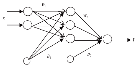
Table 1 shows the ANN architecture used for training. The number of neurons in the input layer is 11 (nine independent variables) because the x 1, x 2, x 3 and x 4 factors correspond to a single independent variable, and are dependent upon each other. For the development of the model, the Mean Square Error (MSE), defined by Eq. (2) and the correlation coefficient (r) were used as the termination criteria.
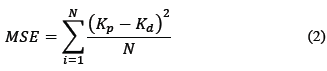

Where k p and k d are the predicted and experimental values, respectively, and N is the total number of data.
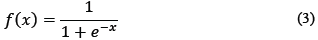
The activation function computes the activity status of a neuron by calculating the global input at an activation value [30]. The most common functions are the sigmoidal logistic function, Eq. (3), and the hyperbolic tangent function, Eq. (4).

In order to improve the behavior of the ANN, the input and output values of the network were standardized using Eq. (5) [31].

Where data norm (i) refers to the standardized data for each i variable, data (i) is the data entered by the user for each i, and amplitude (i) and offset(i) (compensation) are coefficients calculated for each i by eqs. 6, 7.
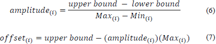
The upper and lower values are the limits of the normalized value, and Max (i) and Min (i) are the maximum and minimum values found within variable i.
2.4. Training and cross-validation
For network training, the commercial software, NeuroSolutions 2016, was employed. The training was performed within the architecture defined in Table 1, varying the number of neurons in the hidden layer and the transfer function. The training process was repeated several times, in order to obtain the lowest MSE. Successful training was achieved when the curve between learning and cross-validation (MSE vs. Epoch) approached zero [32]. Verification was developed with the best weights, stored during training and cross-validation.
2.5. Model
The model is expressed by the matrix in Eq. (8).

Where Y is the array of output variables, f 1 and f 2 are the activation functions in the hidden and output layers, respectively, and X is the input variable array [33].
2.6. ANN performance
ANN performed with through experimental verification values. The MSE, the mean absolute error (MAE) Eq. 9, the Mean Relative Error (MRE) Eq. 10 and the correlation coefficient (r) were used as criteria.
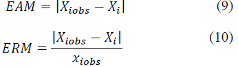
Where, X iobs is the experimental value for i, and x i is the value predicted by the model.
2.7. Sensitivity analysis
The sensitivity analysis was developed in accordance with the methodology established by [33]. This analysis was carried out in order to evaluate the effect of each input variable on the response variable. For this, noise was incorporated into each input variable, using a Gaussian error of 5% (( = 5%) with a 98% probability (the standard adding or resetting value is 2.576( at each input value, taking into account a Box Behnken composite central design (Table 2) with 289 combinations for 11 factors. The entire database (52 data) was assessed, for a total of 165,308 cases.
Table 2 Box-Behnken composite central design for the sensitivity analysis
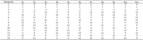
x 1 is the bioactive compound mass (mg); x 1, x 2, x 3 and x 4 is the encapsulating polymeric relationship (e.g. Poly (DL-lactide-co-glycolide) PLGA is a copolymer with two polymers. In this case, the relationship between the copolymer is placed in the variables and if there is no third polymer is placed zero, thus, a 50:50 PLGA would be, x 2=50 x 3=50, and x 4 =0) x 5 polymer concentration (mg/mL water); x 6 polymer mass (mg); x 7 solvent volume (mL); x 8 surfactant concentration (mg/mL water); x 9 emulsion volume (mL); x 10 ultrasound time (min) and x 11 ultrasound power (W)
Source: The Authors.
Finally, the MSE was calculated between the base case (no noise) and the combination of response variables defined in accordance with the design. The average of all MSE's in each run group (Table 2) was plotted.
2.8. Simulation and optimization
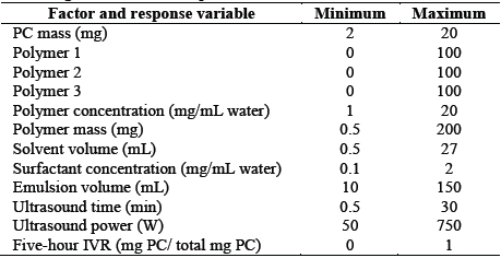
Optimal conditions depend on the final use of the nanoparticle. In this study, the five-hour IVR was maximized. A mixture design with eight factors was used, taking into account the ranges established for each factor (Table 3). R Statistical Software was used.
3. Results and discussion
3.1. Multivariate analysis
The polynomial regression allowed to analyze 7 independent variables for the IVR at 5h and a MSE of 606 (r of 0.17) was obtained. Through this analysis, it could be confirmed that it is not possible to develop a polynomial regression model to correlate mathematically all the factors with the response variable. In addition, the MSE presents very high values and the correlation coefficient is not adjusted. This implies that another methodology is required to obtain a correlation to predict the IVR at 5h. The methodology of ANN has been useful in cases of high complexity because they consider the effect of all the factors on the answer [11].
3.2. Process elements and transfer function in the hidden layer
Table 4 shows the effect of the number of neurons and the transfer function in the hidden layer over the difference between the desired output and that obtained with the model by means of the MSE and r.
Table 4 Effect of the number of neurons and the transfer function over the MSE and r for the IVR at 5h
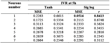
Source: The Authors.
The optimal ANN consisted of a hidden layer with one neuron. The transfer function that allowed to predict the response was Sigmoidal Logistics (eq. (5)). The model presented a MSE of 0.0516 and an r of 0.8413. When performing an analysis of variance, it was noted that the model allows to predict the IVR at 5h of nanoencapsulated PC with a statistically significant generalization (p < 0.05) within the ranges established for the model.
3.3. Model
The mathematical correlation between the factors and the IVR to 5h can be represented by the algebraic system eqs. (11, 12).
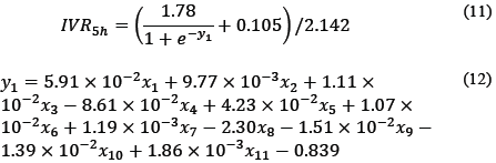
Where, x 1 is the quantity of PC (mg); x 2, x 3 and x 4 is the relationship between encapsulating polymers, x 5 is the concentration of the polymer (mg/mL water), x 6 is the quantity of the polymer (mg); x 7 is the volume of solvent (mL); x 8 is the surfactant concentration (mg/mL water); x 9 emulsion volume (mL); x 10 is the ultrasound time (min), and x 11 is ultrasound power (W).
The algebraic equation system can be easily programmed into a spreadsheet in Microsoft Excel, so as to determine the nanoencapsulated PC IVR at five hours.
3.4. ANN performance
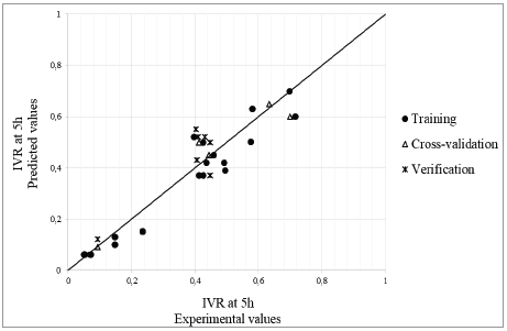
In Fig. 2, the correlation between the values predicted by the model and the experimental values taken for training, cross-validation, and verification are shown. When the AN performance is evaluated with new data for verification, the predicted values approached experimental values, and the training MSE was corroborated. An r of 0.8413, a MAE of 0.1091, and an MRE of 0.1372 were obtained. These results show an approximation to a normal distribution near zero, with 95% probability. The model is capable of predicting, with statistically significant probability (P < 0.05), the IVR at five hours, when the model is processed with new data.
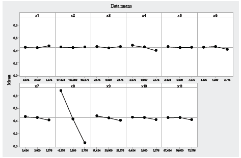
3.5. Sensitivity analysis
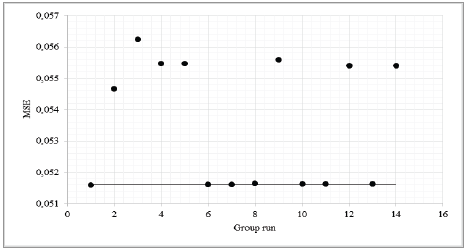
The model presents high sensitivity to surfactant concentration, since all points related to this factor showed an MSE of greater than 0.054 (Fig. 3). The other factors did not have an effect on the model’s sensitivity to "noise". Phenomenologically, this is because the surfactant influences surface tension of the contact surface between the aqueous and the oily emulsion phase. Therefore, it is the one that permits emulsion maintenance, in order to create nanoparticles and release the compound at the required rate [34]. Another explanation for this sensitivity is given by authors including [35, 36] who have proven that there is a connection between principal component analysis and neural networks. These authors suggest that, when a multi-layered perceptron network that learns from a retropropagation algorithm and monitored by a self-associative mode is used to train a neural network, it is possible to obtain a self-organized system, with feed-forward synaptic connections from the factors to the response variables. The strength of network synaptic connections (synaptic weights) is modified in accordance with the response of the neural signal, due to synaptic plasticity in descending order.
Source: The Authors.
Figure 3 Sensitivity analysis for the five-hour IVR model. (-) basic case without “noise”.
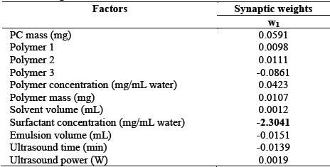
Table 5 shows that, when performing a principal component analysis, the factor that presents the highest absolute weight value is the surfactant concentration, and therefore, this is the factor that presents greatest sensitivity to "noise". This is corroborated by the main effects graph in Fig. 4.
3.6. Simulation
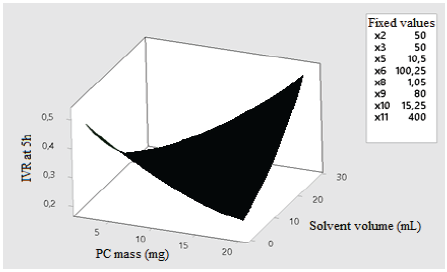
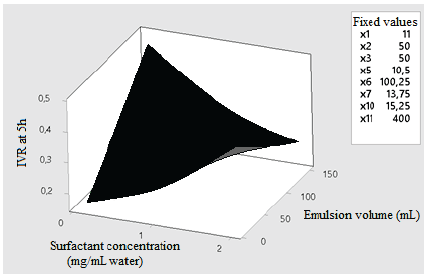
According to the Pareto diagram of standardized effects, factors that have statistically significant effects (p < 0.05) on five-hour IVR include the relation between the PC mass- solvent volume (Fig. 5), and relation between the surfactant concentration-emulsion volume (Fig. 6). Fig. 5 shows that, as the PC mass and solvent volume increases, the IVR also increases because the solvent allows the PC to be scattered throughout the emulsion evenly, which broadens the release. On the other hand, in Fig. 6, it is observed that, as the volume of the emulsion increases at a surfactant concentration between 0.1 and 0.5, the five-hour IVR increases. This is because the IVR depends on several factors at the molecular level, such as the desorption of PC linked to the nanoassembly, the mechanisms of diffusion and erosion of the PC through the nanoparticle, and the chemical composition of the nanoparticle wall.
Source: The Authors.
Figure 5 Effect of the relation between PC mass - solvent volume over the five-hour IVR
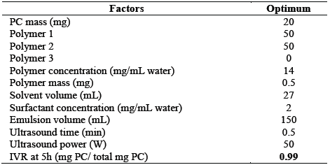
Optimization
A multivariate optimization was performed. Table 6 shows the optimal conditions of the factors that maximize the five-hour IVR. A desirable 0.9996 was obtained. It was observed that it is possible to release a mass fraction of 0.99 of the phenolic compound at that time.
4. Conclusions
The model developed by ANN makes it possible to mathematically correlate the in vitro release five hours after nanoencapsulating phenolic compounds with the PC mass, the relation, concentration, and mass of the encapsulating copolymer, solvent volume, surfactant concentration, emulsion volume, and ultrasound time and power. This model allows for prediction of the response variable with a mean square error (MSE) of 0.0516 and a correlation coefficient (r) of 0.8413, with a statistically significant generalization (P < 0.05).

