


 Inglés (pdf)
 Articulo en XML
 Referencias del artículo
 Enviar articulo por email
 Citado por SciELO
  Citado por Google
  Similares en
SciELO
Similares en
SciELO  Similares en Google
 Permalink
1. Introduction
One of the most influential variables in the process of establishing watershed water balance is surface runoff -- the sheet of water from rainfall which does not seep into the soil and drains onto the surface and that depending on the state and characteristics of the basin moves at different speeds causing various negative effects on watershed management, such as erosion and floods [1]. For this reason, hydrometeorological, hydrological, hydraulic, economic, social and political principles must be integrated into the analysis.
Each basin has unique features that identify and differentiates it from its environment. However, the hydrological processes that develop in each one is similar: precipitation, infiltration, evapotranspiration, and runoff. Precipitation is one of the main climatic variables required for the estimation of water balance; it significantly influences climatic phenomena that may be adverse to society, such as floods.
Modeling and simulation of water balance and flooding variables require the use of technological tools that allow us to distinguish the probable causes of the damage caused in the basin and thus to document the key factors involved in such damages. Among these tools are the hydrodynamic and rainfall-runoff models, which permit to simulate the influence of the spatial distribution of water balance variables and natural properties of the basin on runoff processes [2, 3]. These models are used in combination with geographic information systems (GIS), expanding the range of hydrological investigations, and therefore, the understanding of the fundamental physics of the hydrological cycle processes and the solution of mathematical equations that represent these processes.
In addition, hydrodynamic models can be combined with interpolation methods that allow the interaction of topographical and geographical data, which have been used in various parts of the world to generate maps of water balance variables [4, 5, 6]. These methods use multivariate statistical models that allow evaluating the relationship of climate data with geographical and topographical variables of weather stations and their spatial correlation [5, 6].
This study aims to establish a geostatistical model to predict the magnitude and location of the hydrometeorological variables involved in water balance as precipitation, evapotranspiration, infiltration, runoff and the volume of water stored, including the evaluation of the incidence of antecedent soil moisture conditions in surface runoff produced in the basin.
Estimation of runoff is of great interest for various applications: environmental impact studies, land use planning, management of watersheds and natural resources, prediction of flood risks and implementation of early warning systems [7].
The results of this research will provide basic input for designing a Risk Management Flood Plan, and its implementation will be useful in preventing damage to communities which are located in the flood plains of the 14 main rivers as in the surrounding areas of the three water reservoirs of this basin and that constitute the supply system of the central region of country.
2. Methodology
2.1. Study area
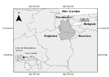
The Pao River basin is located in the North-Central region of the Bolivarian Republic of Venezuela. It has a territorial extension of 3.019 km², distributed among the states of Carabobo, Cojedes and Guárico. It lies between North latitudes 9 ° 33'38 991 ", 10 ° 20' 29.963, and West longitudes 68 ° 17'35 54", 67 ° 48' 319.348" [8, 9].
The geographical location of the Pao River basin in the North-Central region of the Bolivarian Republic of Venezuela by the Caribbean Sea is shown in Fig. 1.
Source: MANR
Figure 1 Geographical location of the Pao River basin in the North-Central region of the Bolivarian Republic of Venezuela by the Caribbean Sea.
The research was carried out in two phases. Phase I involves the geostatistical modeling and Phase II comprises the spatio-temporal modeling of water balance variables of the Pao River basin.
The activities in each phase are described as follows:
2.2. Phase I: geostatistical modeling
The application of geostatistical techniques requires complying with the following steps: 1. Exploratory Analysis, 2. Structural Analysis, 3. Predictions [10].
Using an exploratory analysis, the compliance with the principles of stationarity and extreme outliers are verified, data normality by transformations, evaluation of variable distribution and the existence of correlations among them are identified. The module of Geostatistical Analysis in ArcGis 10.0, is used for producing histograms and determining if the data are fitted a normal distribution function. For a Gaussian distribution of data, the mean and median must be similar, a unit difference between them is accepted. The bias coefficient must be a value between 0 and 0.5. If this is not fulfilled, the data must be transformed [11].
The structural analysis consists of analyzing data to determine its spatial variability, evaluating the presence of anisotropy, and determining variogram models (graphs) for each variable, followed by its validation using the cross- validation technique [12].
By using structural analysis, theoretical models are adjusted to represent the spatial correlation between data (semivariograms), and by using spatial interpolation techniques kriging, the value assumed by the study variables for different points within the region is estimated [13].
In this research, ordinary kriging method was selected, which has been used to model hydrometeorological data in other studies.
The ordinary kriging method is the best linear unbiased estimator, turning it into the optimal technique for the interpolation of any type of spatial variable [14].
The advantage of the ordinary kriging method is the possibility of modeling the spatial dependence of data, and thus, provides the best results among other purely spatial methods in the interpolation of precipitation [15, 16].
The method of ordinary kriging has been used for the application of radar rainfall data for estimating field precipitations for climate purposes. These are some examples of the application of the ordinary kriging estimator as an adequate statistical interpolation method to reliably estimate precipitation values.
The data are represented in an empirical semivariogram and the mathematical models used for their theoretical representation (curve) correspond to Circular, Spherical, Exponential, Gaussian, Bessel-J, K-Bessel, and Stable models, for being the ones commonly employed.
The final step in the geostatistical analysis was forecasting. The setting of the experimental variograms always causes uncertainty on the stationarity assumptions and selected models among others, which contribute to errors in estimation. Therefore, a means to diagnose some problems in the retrieved setting is the use of cross-validation, whose basic idea is to delete a datum in order to predict the deleted observations. If the chosen theoretical model is good or adequately describes the spatial dependence, the predicted value will be close to the real one [17].
The model to be selected is the one that best reproduces the known data; and therefore, will comply with the following conditions: root mean square error (RMSE): the smaller, the better forecasting; standard error of the mean (SEM): small, close to RMSE; the variability of the prediction is calculated correctly and the root mean square error (RMSE): near one (1). If this is fulfilled, the forecast errors are valid.
2.3. Phase II: Modeling of water balance variables
Meteorological data:
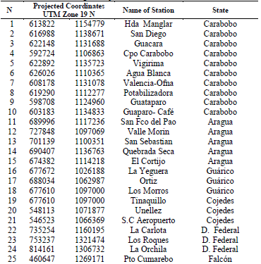
The weather information used in this research is taken from 25 monitoring stations at the six States surrounding the basin, property of the National Institute of Meteorology and Hydrology (INAMEH for its acronym in Spanish).
The data was obtained from the website of institute from January 2015 to December 2017, presented in Table 1.
Satellite data:
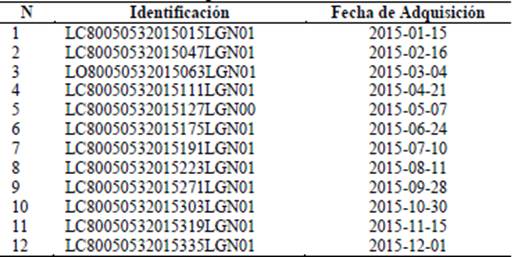
Satellite information was taken from the Landsat satellites L8OLI, for the years 2015, 2016 and 2017, respectively, 36 satellite images were obtained from the web page https://earthexplorer.usgs.gov/ of the United States Geological Service (USGS). The scene used for the Pao River basin is identified under the global reference system according to the following row and path: 005 and 053, respectively.
The map projection parameters according to the USGS are: 1) Projection: UTM, 2) Datum: WGS1984, 3) Ellipsoid: WGS84, 4) UTM Zone: 19 N, 5) cubic convolution as the resampling method.
The data corresponding to the identification and date of acquisition of the satellite images downloaded from the satellite Landsat L8OLI, for the period January - December 2015 are presented in Table 2. As a sample, the identification of the image of satellite Landsat 8 OLI acquired in 2015-01-15 corresponds to the following identification LC80050532015015LGN01.
2.3.2. Data Processing
This study required the use of various techniques and computational tools for the preliminary processing of the Landsat satellite images, which include absolute and relative corrections of each image. The atmospheric, topographic and radiometric corrections applied to each image were executed with the computational tool of satellite image processing known as ENVI 4.7.
For the change detection of use and land cover (LULC) in the basin of the Pao River during the period 2015-2017, the satellite image processing was applied on a multispectral image pixel, being labeled according to the LULC category to which belong. From each image, it was generated thematic cartography and statistical inventory of the area involved in each category. There are two methods of classification: supervised and unsupervised, supervised classification process was used; this type of classification is based on the prior knowledge of classes and statistics that relate to each spectral class of the image. [18, 19] consists of two (2) phases: training and assignment
In phase 1, it was carried out a general recognition of the study area, determining shapes and colors patterns related to a class. By means of pixel training samples it was possible to classify the whole pixel to its corresponded class. The spectral characteristics of bands allow the discrimination of pixel groups that belong to a same LULC class through the generation of their spectral signatures [20]. In phase 2, a list of names or classes is assigned to each pattern observed, by means of algorithms generating a general classification of the image. Once the classification is executed, it is recommended to verify it. For this, a confusion matrix, which includes unclassified/classified pixels, is used as measurement tool. Three types of accuracy were generated with the confusion matrix: global accuracy, accuracy of the user and accuracy of producer [21], as well as the Kappa index [22]. This process is called image classification and it seems to follow the supervised method.
To obtain the losses and estimate the surface runoff from them, the method of the U.S. Soil Conservation Service was used [23].
This method requires to know the type and use of the basin soil studied to determine curve number, pluviographic records, and other factors such as the time elapsed since the last rainfall and evapotranspiration during the period of study.
In this investigation, water balance was expressed according to the following equation:

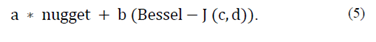
Where ΔS represents the variation of water stored in the soil (mm); I represents the infiltration in (mm); ETR evapotranspiration in (mm). It is considered that
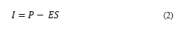
Where P represents precipitation (mm); ES represents the surface runoff (mm).
3. Results
The results that encompass the creation of variable maps using GIS techniques are the following: a) LULC, b) precipitation, c) evapotranspiration, d) infiltration, e) effective precipitation, and (f) storage of water volume.
With regard to the phase I of investigation which corresponds to geostatistical modeling it was observed that the behavior of the data of rainfall reported by the network of weather stations used in this study reported a mean of 16.8 and a median 16.4, with a coefficient of asymmetry of 0.25, which confirms a behavior of normal distribution of the data, the trend that follows the distribution of the data is of second order which. It will be removed in the structural analysis. The behavior of the hydrometeorological variables presented non-stationarity with respect to the X-axis, and y Z. In addition to an anisotropic behavior. Table 3 shows the models and forecast errors.
Table 3 Models and forecast errors
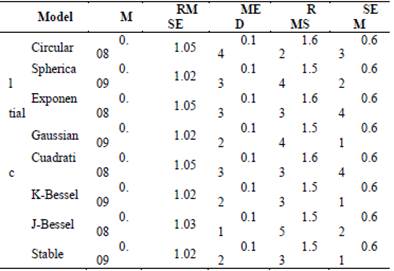
(RMSE) root mean square error; (SEM) standard error of the mean; (RMS) root mean square (RMS).
Source: The Authors.
According to this analysis, the Bessel-J model was selected since it best fitted the values of the variables to be studied in this research.
3.1. Land use and cover
The types of soils present in the basin were determined from the soil map obtained from the website of the Ministry of Environment and Natural Resources prepared for the Bolivarian Republic of Venezuela, the results in Fig 2 show the presence of four types of soil: 1) Oxisol (13.30%), 2) Inceptisol (60.21%), 3) Mollisol (5.92%) and (4) Ultisol (20.5%). As a sample, the mean of the amount of organic carbon at different depths of the profiles in the order inceptisols is varying between 1.1 and 1.44% to 0-15 cm soil depth [24]. The distribution of inceptisol soil particle size corrsponded to a depth of 0 to 24 cm determined by [25] corresponds to: sand: 70.45%, silt: 15.06%, clay: 14.49%. The mean amount of organic matter and mean texture [26, 27] determine the type of soil of the mollisols as follows: organic matter: 26 g / kg (2.71%), sand: 120 g / kg (12.5%) silt: 577 g / kg (60.16%), clay: 236 g / kg (24.6%). As it can be seen, the soils of Pao River basin have predominantly contained particles of fine and finest, being considered as class C (moderately high runoff) and D (high runoff) according to the hydrologic classification of US-SCS.
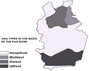
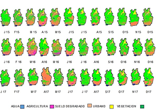
Fig. 3 shows the results from the application of change detection techniques in areas destined for land use and cover of the Pao River basin corresponding to the post-classification comparison method from to January 2015 to December 2017. The result of the kappa index to validate the classification carried out is in the category of satisfactory compared with the level of concordance of [28]. For other authors, kappa represents the value of K or strength of concordance, the retrieved value falls in the range from 0.81 to 1, which is classified as very good.
Source: The Authors.
Figure 3 Use and land cover in the basin of the Pao River in the period from 2015-2017.
A more detailed investigation of this use of the Pao River basin land classification can be reviewed in [29].
3.2. Precipitation
The area studied has two climatic seasons [30]: a dry season corresponding to the months from December to March with low-intensity monthly precipitations ranging from 0 mm/month to 48 mm/month, and a rainy season from April to November with a monthly precipitation varying from 11.58 mm/month to 419.96 mm/month.
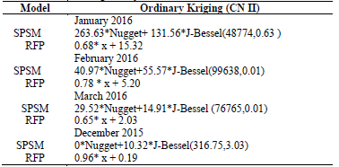
Table 4 Results of the spatial prediction statistical modeling of monthly rainfall in the dry season for 2016.
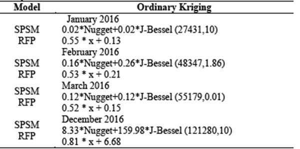
(SPSM) Spatial prediction statistical model. (RFP) Regression function Prediction.
Source: The Authors.
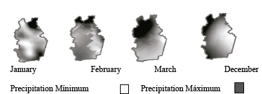
Fig. 4 represents a sample of the results from the monthly precipitation in mm/month during the dry season for 2016. It is observed for January (0.095-0.740), February (0.071-0.745), March (0.051-1.669), December (28.31-45.2). For 2016, the mean precipitation was of 13.60 mm/year in the dry season and 282.92 mm/year in the rainy season.
Source: The Authors.
Figure 4 Spatial prediction of monthly precipitation (mm/month) occurring in the Pao River basin in the dry season for 2016.
The information shown in Table 4 corresponds to the results of the spatial prediction statistical modeling of precipitation from the dry season in the Pao River basin for 2016.
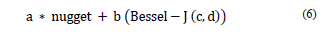
The spatial prediction statistical model (SPSM) used is the Bessel-J function. The equation is expressed as follows:

Where the coefficient a is associated with the non-spatial correlation; the coefficient b is associated with the term C0 +C1,which is the threshold variation; the coefficient c represents the maximum distance between neighboring precipitation observation stations; and the coefficient d represents the parameter of the Bessel-J function. The coefficient values vary as follows Table 4a: between 0.01 and 8.331,b: between 0.0233 and 159.98,c: between 27431 and 121280,d: between 0.01 and 10. A pattern for the semivariances of the SPSM for the dry season associated with the first months of each year is observed. In all cases, the semi variances are smaller in the shortest distance and then stabilize at a certain distance.
3.3. Evapotranspiration
The area studied has two seasons: a dry season corresponding to the months from December to March with a monthly evapotranspiration presenting a high intensity spatial distribution, which reaches up to 1372.64 mm/month; and a rainy season from April to November with a monthly evapotranspiration ranging from 0.00 mm/month to 3627.8 mm/month.
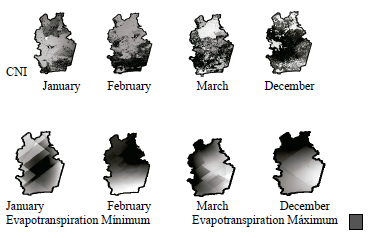
Fig. 5 represents a sample of the results from the monthly evapotranspiration in mm/month during the dry season for 2016. It is observed for January (0.00-269.35), February (130.40-153.77), March (159.89-185.47), and December (84.68-109). For 2016, the average evapotranspiration was of 179.39 mm/year in the dry season and 134.42 mm/year in the rainy season.
The information shown in Table 5 corresponds to the results of the spatial prediction statistical modeling of evapotranspiration based on the dry season in the Pao River basin for 2016.The spatial prediction statistical model (SPSM) used is the Bessel-J function. The equation is expressed as follows:

Where the coefficient a is associated with the non-spatial correlation; the coefficient b is associated with the term C0 +C1, which is the threshold variation; the coefficient c represents the maximum distance between neighboring precipitation observation stations; and the coefficient d represents the parameter of the Bessel-J function correlation especially. The coefficient values vary as follows Table 5a: between 9.658 and 200.81,b: between 59.797 and 830.84,c: between 57539 and 135640,d: between 0.01 and 4.39. A pattern in the SPSMs for the dry season associated with the first months of each year is observed. In all cases, the semivariances are smaller in the shortest distance and then stabilize at a certain distance.
Table 5 Results of the spatial prediction statistical modeling of the monthly evapotranspiration during the dry season for 2016.
Source: The Authors.
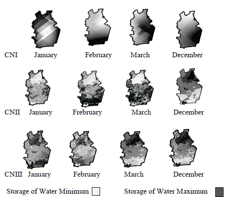
3.4. Infiltration
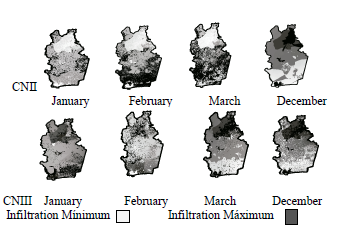
Fig. 6 represents a sample of the results from the monthly infiltration expressed in mm/month for different soil moisture conditions: dry (CNI), normal (CNII) and wet (CNIII). Taking as an example the dry season for 2017, infiltration values are as follows: January: CNI (0.0189-148.245); CNII (0.00-129.54); CNIII (0.0189-91.5297). February: CNI (0.0-43.972); CNII (0.00-25.912); CNIII (0.00 - 26.047). March: CNI (0.00-48.06); CNII (0.00-47.41); CNIII (0.0-45.743). December: CNI (0.00-95.81); CNII (0.00-94.21); CNIII (0.00-73.90). During the rainy season for 2017, an increase in infiltration without any significant differences regarding variations of humidity conditions was observed. The máximum average of infiltration was 227.92 mm.
Source: The Authors.
Figure 6 Spatial prediction of monthly infiltration (mm/month) modifying the Pao River basin soil moisture conditions during the dry season for 2017.
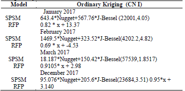
The information shown in Table 6 corresponds to the results of the spatial prediction statistical modeling of infiltration according to the dry soil moisture condition (CN I) during the dry season in the Pao River basin for 2017.
Table 6 Results of the spatial prediction statistical modeling of monthly infiltration during the dry season for 2017.
Source: The Authors.
The spatial prediction statistical model (SPSM) used is the Bessel-J function. The equation is expressed as follows:
Where the coefficient a is associated with the non-spatial correlation; the coefficient b is associated with the term C0 +C1, which is the threshold variation; the coefficient c represents the maximum distance between neighboring precipitation observation stations; and the coefficient d represents the parameter of the Bessel-J function. The coefficient values vary as follows Table 6a: between 26.57 and 1469.5;b between 29.47 and 567.76c: between 4202.2 and 23684, d: 3.5148 and 4.82
A pattern in the SPSMs for the dry season associated with the first months of each year is observed. In all cases, the semivariances are smaller in the shortest distance and then stabilize at a certain distance
3.5. Effective precipitation
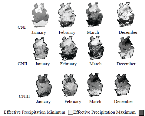
Fig. 7 represents a sample of the results from the monthly effective precipitation expressed in mm/month for different soil moisture conditions: dry (CNI), normal (CNII) and wet (CNIII).
Source: The Authors.
Figure 7 Spatial prediction of effective monthly precipitation (mm/month) modifying the Pao River basin soil moisture conditions during the dry season for 2015.
Taking as an example the dry season for 2015, the effective precipitation values are as follows: January: CNI (3.36-34.62); CNII (3.36-25.94); CNIII (0.091-45.5). February: CNI (0.010-45.5); CNII (6.58-45.5); CNIII (0.09-45.5). March: CNI (0.629-28.70); CNII (2.44-14.60); CNIII (0.0-4.656). December: CNI (0.00-45.5); CNII (0.441-22.82); CNIII (0.00-45.5).
During the rainy season for 2015, an increase of effective precipitation without any significant differences regarding variations of humidity conditions was observed. The máximum average of surface runoff was 164.11 mm.
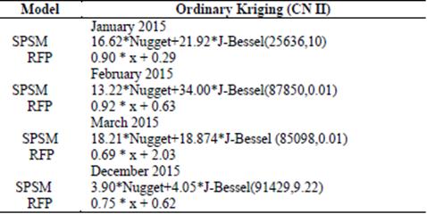
The information shown in Table 7 corresponds to the results of the spatial prediction statistical modeling of runoff according to normal soil moisture conditions (CN II) during the dry season in the Pao River basin for 2015
Table 7 Results of the spatial prediction statistical modeling of monthly runoff during the dry season for 2015.
Source: The Authors.
The spatial prediction statistical model (SPSM) used is the Bessel-J function. The equation is expressed as follows:
Where the coefficient a is associated with the non-spatial correlation; the coefficient b is associated with the term C0 +C1 which is the threshold variation; the coefficient c represents the maximum distance between neighboring precipitation observation stations, and the coefficient.d represents the parameter of the Bessel-J function.
The coefficient values vary as follows Table 7a: between 3.90 and 18.21,b: between 4.05 and 34.00, c:between 25636 and 91429, d:between 0.01 and 10. A pattern in the SPSMs for the dry season associated with the first months of each year is observed. In all cases, the semivariances are smaller in the shortest distance and then stabilize at a certain distance.
3.6. Storage of water volume
Fig. 8 represents a sample of the results from the monthly storage of water volume expressed in mm/month for different soil moisture conditions: dry (CNI), normal (CNII) and wet (CNIII).
Source: The Authors.
Figure 8 Spatial prediction of monthly storage of water volume (mm/month) modifying the Pao River basin soil moisture conditions during the dry season for 2016.
Taking as an example the dry season for 2016, storage of water volume values are as follows: January: CNI (- 2.693-21.0); CNII (- 2.693-21.0); CNIII (- 2.693-21.0). February: CNI (- 153.7, - 130.4); CNII (- 153.7, - 130.4); CNIII (- 153.7, - 130.4). March: CNI (- 185.4, - 159.8); CNII (- 185.4, - 159.8); CNIII (- 185.4, - 159.8). December: CNI (- 109.8 - 84.68); CNII (- 109.8, 84.68-); CNII (- 109.8, - 84.68).
During the rainy season for 2016, an increase in the storage of water volume without any significant differences regarding variations in humidity conditions was observed. The maximum average of storage of water volume was - 88.46 mm.
The results presented a storage deficit is this basin for 2016 and 2017.
The information shown in Table 8 corresponds to the results of the spatial prediction statistical modeling of the monthly storage of water volume during the dry season in the Pao River basin for 2016.
Table 8 Results of the spatial prediction statistical modeling of the monthly storage of water volume during the dry season for 2016
Source: The Authors.
The spatial prediction statistical model (SPSM) used is the Bessel-J function. The equation is expressed as follows:
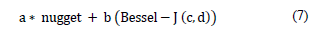
Where the coefficient a is associated with the non-spatial correlation, the coefficient b is associated with the term C0 + C1, which is the threshold variation the coefficient c represents the maximum distance between neighboring precipitation observation stations, and the coefficient d represents the parameter of the Bessel-J function.
The coefficient values vary as follows Table 8 a: between 0 and 263.63, b: between 10.32 and 131.56, c: between 316.75 and 99638,d: between 0.01 and 3.03.
A pattern in the SPSMs for the dry season associated with the first months of each year is observed. In all cases, the semivariances are smaller in the shortest distance and then stabilize at a certain distance.
4. Discussion of results
The post-classification comparison method results in five classes: a) water, b) agriculture, c) degraded soil, d) vegetation and e) urban area. The Pao River basin shows the presence of vegetation with 75.43%, represented by bushes, forests and natural grasslands grazed [31], and agricultural use 12% as classes predominantly during the rainy season, while average urban area in 3.7% and 1% water. While the dry season is dominated by the presence of degraded soils by 55%, 8% agricultural use, the urban area is maintained at an average of 3.6% and water at 0.8%.
The existence of degraded soils as a result of indiscriminate deforestation for traditional farming of smallholdings that has led to a loss of the original vegetation cover was observed [32].
Regarding precipitation, the results show that the rainy season concentrates more than 85% of the total annual precipitation, while in the dry months it barely rains with a monthly precipitation below the reference evapotranspiration [33].
Monthly watershed infiltration was evaluated according to soil moisture conditions: condition I for dry soil, condition II for normal soil, and condition III for moist soil. During the period studied in this research, the infiltration parameter values obtained are low, closer to the minimum value. No significant differences in accordance with diverse soil moisture conditions are observed [34].
In the basin of the Pao River, for the purposes of estimation of infiltration and runoff most of the area is occupied with soil organic silt, silty sand and silty clay that corresponds to soils of moderate potential for runoff (hydrological groups C and D) the values from the variable surface runoff makes that the relative grade it means almost throughout the basin, which responds to the vegetation cover in rainy season and the reported values deficit of storage in the basin [31].
Runoff values range from 0.0 to 370 mm / year in 2015; 0.0mm to 389 mm/year in 2016, and 0.0 to 312 mm per year in 2017, these values indicate the potential amount of precipitation which can lead to flooding in the basin, this parameter is important in this research since it is an input for the design of a risk management Plan flooding in the basin. The distribution of the storage in the soil derived from water balance modeling allows to spatially predicting that the trend is towards the occurrence of water charging towards the mountains that delimit the Pao River basin, mainly in the Northern area (Fig. 8).
By representing the data in an empirical semivariogram and adjusting it to the mathematical models used for its theoretical representation, it was possible to compare the prediction error results. For this research, the Bessel-J model was selected, representing a novelty of the method using hydrometeorological variables, since the literature reports the use of other models. This represents a contribution of this research to the understanding of this type of hydrometeorological variables, which can be applied to operating forecasts and actions of prevention of flooding in high-risk areas.
5. Conclusions
In this study, based on a spatio-temporal data modeling using satellite image analysis and processing and geostatistical methods, a spatial prediction statistical model was found for water balance variables in a basin of Venezuela. In addition, the different soil moisture conditions of the basin were combined. The results show an acceptable fit of the variables involved in the model: 1) precipitation, 2) evapotranspiration, 3) infiltration, 4) effective precipitation and 5) storage of water volume.
Spatial prediction of water balance shows a trend in the occurrence of recharge in areas north and south of the basin of the Pao River, favoring permanent water supply to three reservoirs for the purpose of supplying human located in sectors of the high, middle and lower basin of the Pao River.
The technique used for the determination of the effective rain is very useful in the forecasting of the temporal variation of the surface runoff of a basin for hydrological engineering and flood control, and identification applications of flood area. The use of remote sensing and GIS can provide the right platform to converge a great volume of multidisciplinary, being also an economic technique data. The spatial prediction statistical model of the semivariances for surface water balance (SWB) was the Bessel-J model. The correlation coefficient (R) values obtained for the statistical models of SWB spatial prediction vary according to the following ranges: precipitation 0.54-0.81; evapotranspiration 0.53-0.86; infiltration 0.68-0.95; runoff 0.68-0.92; and storage of water volume 0.53-0.95.
These values confirm that the method used to generate spatio-temporal predictions is suitable. Regarding to the evaluation of the incidence of antecedent soil moisture conditions in runoff production, the results allow to conclude that the inclusion of the antecedent moisture condition does not report significant changes in the final results for assessing surface runoff production as an important factor in hydrological studies since it determines the flooding risk factor for the communities and activities located on the floodplains of basin.

