


 Inglês (pdf)
 Artigo em XML
 Referências do artigo
 Enviar este artigo por email
 Citado por SciELO
  Citado por Google
  Similares em
SciELO
Similares em
SciELO  Similares em Google
 Permalink
1. Introduction
Productivity, together with the protection of natural resources, depends on an effective and efficient intervention of agroecosystem, critical aspects to achieve its viability and sustainability. Ecosystems are composed of a series of elements in constant interaction; therefore, a change in any of them can mean a variation in the others, given the multiplicity of relationships exhibited. In the agricultural context, it is clear that various factors such as topography, soil, climate, pests and diseases, and the genetics of plants are influencing yield under similar management strategies [1]. Due to the high variability of factors - even on a small scale - along with farming, homogeneous management practices do not always allow high yields [2], on the contrary, they contribute to the inefficiency of the system due to under or overuse of supplies increasing management costs and energy waste [3].
Precision agriculture has the objective to implement differentiated practices according to the specific requirements of each management zone based on the ability to express intra and inter management zones, complex relationships between factors determining crop yield [4]. The essential issue consists of the identification and spatial delineation of uniform fields, which must represent a similar combination of factors that are potentially limiting yield [5]. In several investigations related to precision agriculture, the spatial analysis of soil properties has allowed delineating management zones; physical and chemical properties of the soil have been the most used, meaning that rates supply may be improved, as well as the viability of site-specific management, when compared with the homogenous management strategy [6,7]. The delineation of site-specific management zones usually begins with a pre-established diagnosis of soil properties; they rarely associate in situ with yield because many of them are not limiting factors [3] for which homogenous management strategy is the best option. The multiple soil properties related to yield hinder the discrimination in limiting and not limiting factors. Therefore, the isolated description of one of them does not provide sufficient information to explain the productive response of a crop nor indicate which factors require site-specific or homogenous strategies management. Univariate analysis methods are still accepted to describe multivariate systems, such as those that occur in the continuous soil-plant-atmosphere, however, to understand the functioning of this complex system, the simultaneous study of multiple factors is required. Multivariate analytical techniques [8] are useful tools to accomplish this purpose of a scenario in which various factors converge, such as that presented in the soil-plant system [9]. Several authors used the multivariate data analysis approach to study the interaction of soil properties [10, 11] as well as its relationship with crops yield [12]. These techniques allow dimensional reduction of a multivariate phenomenon, promote the associations between crop components, the visualization of high-intensity patterns, and intuitive results representations [13].
The objective of the work was to delineate management zones identified by multivariate analysis of a set of soil properties and crop yield components, as a tool in the definition of the site-specific management strategy.
2. Materials and methods
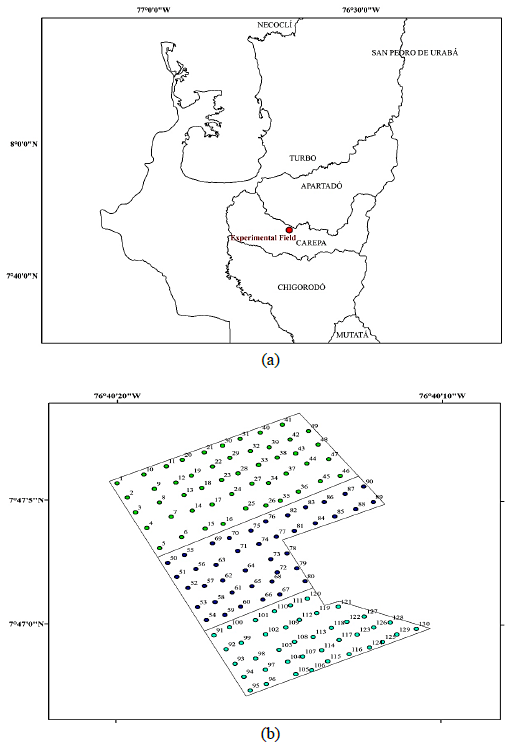
The work was performed in an experimental banana field located in the municipality of Carepa, west Colombia (Fig. 1a). The field soil belongs to the consociation loam fine Vertic Endoaquept and the tropical humid forest climate. It has seven lots established since 2005 with clone Williams, a type of banana from the Cavendish AAA group, sowed at 2.5 m distance between plants and rows. In the middle of the field, 130 banana production units were located in a regular grid of 20 x 20 m, comprising an area of six hectares, and three plots of the farm (Fig. 1b). The places were georeferenced with a Trimble GeoXT GPS set with the WGS84 datum and the projection system UTM zone 18 N.
Source: The Authors.
Figure 1 Geographic maps. (a) Location of the experimental field in relation to the municipalities of the banana zone in Uraba, Colombia. (b) Experimental field and sampling sites identified by their number (1-130) and lot (lot 3: green, lot 4: blue, lot 5: cyan).
2.1. Field sampling and laboratory determination of variables
Yield. One production unit was labelled (three plants of three consecutive generations per place) in each referenced site. One sucker was selected from the cylinder of the tuberous rhizome and the others were eliminated in order to equal the plants of the third generation of the units in growing and cultivation until plant production. Nine production descriptors and two describing the functionality of the plant root at harvest moment were determined for each harvested bunch and regarded as dependent variables (Table 1). Soil properties. When the flowering of fifty percent of the plants occurred, nineteen physical properties were measured at the cardinal points of the production unit. Seventeen chemical properties were determined on a composite sample formed by four sub-samples extracted from the cardinal points of each plant and operated also as explanatory variables. Table 2 shows the chemical and physical procedures followed
Table 1 Physiological and Yield descriptors
| Yield component or physiological descriptor | Code | Unit |
|---|---|---|
| Total bunch weight (Production) | Pr1 | kg |
| Exported bunch weight | exportado | kg |
| Rejected bunch weight | rechazo | kg |
| Bunch hands number | manos | # |
| Bunch fingers number | dedos | # |
| Central finger width of the second hand | Vmano2 | cm |
| Central finger width of penultimate hand | Vpenul | cm |
| Central finger length of the second hand | Lmano2 | cm |
| Central finger length of penultimate hand | Lpenul | Cm |
| Functional and not functional root [14] | rf | % |
Source: The Authors.
Table 2 Soil properties and evaluation methods
| Properties | Code | Methods | Unit |
|---|---|---|---|
| Physical | |||
| Texture evaluated on a sample composed of four subsamples taken orthogonally at 30 cm from the plant and between 0 - 20 cm depth. Dispersed clay and dispersion coefficient (CD = ArD/Ar * 100) | A | Texture determined by Bouyoucos method [15]. ArD determined by pipette method [16] | % |
| L | |||
| Ar | |||
| ArD | |||
| CD | |||
| Surface penetration resistance determined at 30, 60 and 100 cm depth | CP30, CP60, CP100 | Pocket penetrometer | kg cm-2 |
| Surface apparent density at 30 cm from the plant | Da | Bevelled cylinder | gr cm-3 |
| Structural stability indexes, evaluated on an undisturbed sample taken at 30 cm from the plant | |||
| Wet and dry mean weight diameter | DPMH | Dry and water sieving according to methods described in [16] | mm |
| DPMS | |||
| Wet and dry structure index | IEH | % | |
| IES | |||
| Wet and dry fine aggregates (< 0.5 mm) | AFH | ||
| AFS | |||
| Wet and dry extreme aggregates (> 2 mm y < 0.5 mm) | AEH | ||
| AES | |||
| Moisture indexes, evaluated on a sample taken at 30 cm away from the plant | |||
| Gravimetric moisture retention at field capacity (0.3 atm) and permanent wilting point (15 atm) | H0.3 | Desorption of moisture in plates and pressure cookers with oxygen | % |
| H15 | |||
| Chemical | |||
| Properties evaluated on a sample composed of four subsamples taken orthogonally at 30 cm from the plant and between 0 - 20 cm depth | |||
| pH | pH | Water 1:1 | - |
| Organic matter content | mo | Walkley-Black [15] | % |
| Effective cation-exchange capacity | CICE | Cation sum | cmol(+) kg-1 |
| Effective cation exchange capacity at pH 7 | CIC7 | Neutral 1N ammonium acetate [15] | |
| Ca | Ca | Interchangeable contents. Ca, Mg and K extracted with neutral 1M ammonium acetate. Al extracted with KCl [15] | cmol(+) kg-1 |
| Mg | Mg | ||
| K | K | ||
| Al | Al | ||
| Ca/Mg ratio | Rel.1 | Ca/Mg | - |
| (Ca + Mg)/K ratio | Rel.2 | (Ca + Mg)/K | - |
| P | P | P: Bray II. S: monocalcium phosphate 0.008M. Fe, Mn, Cu and Zn: Olsen modified. B: hot water. [15] | mg kg-1 |
| S | S | ||
| Fe | Fe | ||
| Mn | Mn | ||
| Cu | Cu | ||
| Zn | Zn | ||
| B | B | ||
Source: The Authors.
2.2. Statistical Analysis
The exploratory analysis of the database was executed partially following the protocol proposed by [17], then a Principal Component Analysis (PCA) was carried out starting from the correlation matrix. This analysis was performed and represented graphically with the "vegan" package [18], generating two forms of visualization of sites and descriptors in the dimensionally reduced space. The first one is the Scaling 1 graphic, where the direction of the vectors representing each variable reflects the linear relationship between descriptors, and the length describes its contribution in the main component. In the Scaling 2 graphic, the scoring of the sites was scaled to the relative eigenvalue, forming a representation whose approximation in the multidimensional space is equivalent to the Euclidean distance. Additionally, each site was categorized with a characteristic shape and colour depending on the quartile of the Production response variable, considered the most significant.
For those vectors that allowed visually discriminating the sites classified by their production quartile, the non-redundant explanatory variables were selected. For this purpose, the analysis of several main components was necessary according to the proportion of variability explained by each of them. The selected variables helped in the elaboration of a Principal Coordinates Analysis (PCoA). This multivariate technique allows a Euclidean representation of a set of objects whose relation is measured by any coefficient of similarity or distance [19]. We verified if the chosen variables allow a suitably discerning of yield or the spatial conformation of the lots. This procedure was executed with variables adjusted to mean zero and variance one, the Euclidean distance was chosen as dissimilarity coefficient.
Dissimilarity coefficients were the input for clustering sites in the Agglomerative Analysis (Cluster), a conventional hierarchical agglomeration strategy was used producing sequential partitions and heuristic clustering criterion [20]. The highest correlation index, obtained through dissimilarity coefficients, allowed selecting the best grouping of sites [21]. The number of groups was determined considering the total average width of the silhouette using the "cluster" package [22,23]. Similarly, variables were analysed through the conformation of spatial distribution charts categorized by their respective quartiles. The main characteristics of the groups and clusters were highlighted with the scattering graphs implementing the package "ggplot2" [24]. A comparative analysis of the Production response variable among groups was carried out to assess their viability. The Correspondence Analysis (CA) allows visualizing the relation of dependence among groups and production quartiles; this analysis starts from a contingency table including the group allocation and production quartile of each site.
The package "ca" was used to implement and represent CA [25], besides, the quantitative differences among groups were analysed based on the spatial behaviour of the variable. For each group, a variogram was elaborated to identify the presence of spatial structure using the "GeoR" package [26], however, due to the absence of spatial structuring, the differences of yield among groups were analysed through an analysis of variance (ANOVA) and Tukey means comparison test with α = 0.05. All the cited packages work in the language and environment R for statistical computing [27].
3. Results and discussion
3.1. Variable selection and group creation
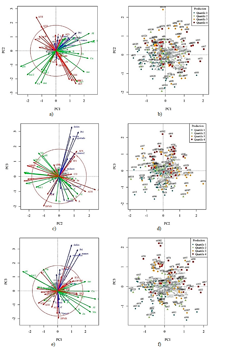
Eleven principal components are required to explain at least 70% of the total variability (Table 3). The linear relationships between variables, as well as site ordering, were showed graphically with principal components. Fig. 2a and b show the association variables with the first two principal components. In these, an inverse relationship between the Production variable response with calcium and pH, but direct with Al, Fe, and Mn is evident. Consequently, these two groups of variables are also showing an antagonistic relationship between them, a logical response in most soils but not expected with yield. In tropical conditions, several studies have demonstrated the adverse influence of aluminium, acidity, and high concentration of iron and manganese in the production [28].
Table 3 Principal Component Importance
| Principal Component | PC1 | PC2 | PC3 | PC4 | PC5 | PC6 | PC7 | PC8 | PC9 | PC10 | PC11 |
|---|---|---|---|---|---|---|---|---|---|---|---|
| Eigenvalue | 6.78 | 5.13 | 3.2 | 3.06 | 2.74 | 2.38 | 2.21 | 1.91 | 1.77 | 1.54 | 1.32 |
| Proportion Explained % | 15.16 | 11.73 | 6.94 | 6.57 | 5.86 | 5.26 | 4.70 | 4.07 | 3.77 | 3.28 | 2.82 |
| Cumulative Proportion % | 15.16 | 26.89 | 33.83 | 40.4 | 46.26 | 51.52 | 56.22 | 60.29 | 64.06 | 67.34 | 70.16 |
Source: The Authors.
This unexpected yield and soil characteristic relationships are showing an imbalance of soil alkalinity respect to other nutrients derived from over-liming. Fig. 3 shows that production units belonging to the lowest production quartile tend to have the highest pH values, although differences are not significant. On the other side, the inverse relationship between the ratio (Ca+Mg)/K (Rel.2) and production (Pr1), are supporting the idea that potassium is unbalanced regarding calcium and magnesium. The strength disequilibrium among cations seems to be playing an influential role in data variability, given the similar form of these variables observed on the graphics components 1-3 (Fig. 2)
Source: The Authors.
Figure 2 Principal components association. (a) and (b) components 1 and 2; (c) and (d) components 1 and 3; (e) and (f) components 2 and 3. In (a), (c), (e) relation of variables labeled by colors; blue for yield, green for chemical, and red for physical soil variables. In (b), (d), (f) scoring of sites categorized by its production quartile.
The imbalance happens because the excessive addition of one nutrient hinders the assimilation and functioning of others. The antagonism reported is a common effect between ions due to similar chemical properties as in the case of calcium, magnesium and potassium [29]. In the banana crop, potassium is the most absorbed nutrient and it is particularly sensitive to soil cation balance [30].
The physical variables in the component space 1-2 show a high degree of a direct or indirect relationship between them. We chose the dry mean weight diameter (DPMS) as a physical variable to explain yield, the highest inverse relation is shown in components 1-3 and 2-3, and to avoid redundancy by including other physical variables (Fig. 2 c-f). This property also allows differentiating yield quartiles, it is an indicator of the state of soil structure, and its inverse relationship with yield indicates that areas with large aggregates are influencing bunch weight negatively.
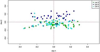
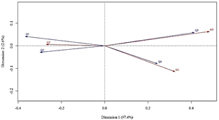
The field has soil with vertic properties, so variability grade in these soils is conditioning the size of the aggregates. These soils have remarkably coarse structural components, separated in dry periods by a large concentration of cracks. Crack swelling in dry periods has adverse effects as breaking of absorbent roots, thick profile desiccation, compaction, and increase in apparent density. Additionally, the DPMS is related to permeability and it is an indicator of soil erosion [31]. Besides the selected variables (Ca+Mg)/K and DPMS, we decided to include pH, although it is strongly related to Ca, Mg, K and their proportions, it is possible to find sites with balance or unbalance of cations at the same pH. The variables (Ca+Mg)/K, DPMS, and pH in the Principal Coordinates Analysis (PCoA) did not allow us to discriminate sites by their production quartile, resulting in a scarcity of a strong association of variables and yield. However, it allowed separating lots to some degree, as shown in Fig. 3.
Source: The Authors.
Figure 3 Principal coordinate analysis with explanatory variables (Ca+Mg)/K - DPMS - pH.
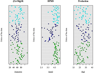
For example, lot 4 differed from the others and there is some grouping degree between lots 3 and 5, showing a relationship between variables and spatial conformation of the sites, relevant aspect of management zones definition. Another way to conceive this association is from the Cleveland plot of Fig. 4.
Source: The Authors.
Figure 4 Cleveland dot plot of explanatory variables (Ca+Mg)/K, DPMS and response variable Production. Data are categorized by their plot as follows: lot 3 = green, lot 4 = blue, and lot 5 = cyan.
The magnitude of variables, according to the reading order of the database, shown in Fig. 1b, creates non-random behaviour in them. The clear trends in lot 3 for the three selected variables stand out, with a significant convergence between production data patterns and the cation ratio. On the other hand, lot 4 has sites with the lowest DPMS, (Ca+Mg)/K ratio and higher yield. These different forms of relations among variables between lots imply different scales of spatial arrangement.
Fig. 5a describes the spatial arrangement of sites according to their group (Cluster), it evidences an aggregate distribution, mainly exhibited in groups 1 and 2. Grouping sites is a desirable condition given the interest of determining management areas to improve inputs and human resources. Additionally, Fig. 5b shows yield distribution classified by its quartile; the similarity allocation pattern of sites stands out, especially in the central sector of the crop and the north-south diagonal.
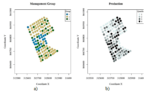
Source: The Authors.
Figure 5 Spatial distribution of the cluster according to: A. Explanatory variables (Ca+Mg)/K - DPMS - pH, and B. response variable production categorized by its quartile.
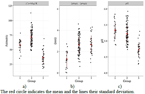
The behaviour of variables related to yield shows that group 2 is composed of the highest imbalance (Ca+Mg)/K ratio, despite having similar pH values as group 1 (Fig. 6 a-c). On the other hand, group 3 has both the lowest cation ratio and pH. Fig. 6b shows the difference of soil aggregates evaluated in dry (DPMS) and wet (DPMH) undisturbed samples. Group 1 presents the lowest magnitude difference between DPMS and DPMH, indicating more stability of dry aggregates in front of water as a disruptor agent. Primary soil particles conform to soil aggregates, which remain stable by the cohesion of secondary particles, resisting disruptive forces. When the difference between these two parameters is lower, there is a sign of structural stability [15].
3.2. Assessment of groups according to yield response
We evaluate the sensibility of the groups formed with soil variables most related to bunch weight to predict spatial yield behaviour. Table 4 shows the contingency table used for correspondence analysis (CA), classifying each site according to its group and respective production quartile. Based on the chi-square (P< 0.05), there is a dependence between groups and quartiles, also evidenced in the CA graphical representation in Fig. 7. In group 2, sites with production in the first two quartiles predominate, while the places of groups 1 and 3 are associated with the upper quartiles suggesting that the edaphic characteristics selected are influential in the yield response of the banana crop.
Source: The Authors.
Figure 7 Correspondence analysis of groups and sites production quartile. Q (blue) = Quartile, G (Red) = Group.
Table 4 Contingency table of groups and production quartile assignation
| Classification | Group | |||
| 1 | 2 | 3 | ||
| Production Quartile | 1 | 3 | 26 | 4 |
| 2 | 4 | 24 | 4 | |
| 3 | 7 | 14 | 13 | |
| 4 | 7 | 15 | 9 | |
Source: The Authors.
The spatial structure of yield was evaluated in each group using a variogram as a statistical tool. All groups evidenced not spatial autocorrelation, where the nugget effect was like the sill, indicating a random variation [32].
The same data was examined in all lots at the time and an anisotropic spatial dependence was found in yield [33]. The random behaviour exhibited by production in each group indicates both an adequate plant clustering and the capture of spatial variation. The strategy allows delineating zones in the field for each group of plants and proposing them as homogenous management zones. The absence of spatial auto-correlation within groups satisfies the assumption of independence. The analysis of variance showed that group 1 has the highest average bunch weight with 33.04 kg, followed by group 3 (32.5 kg), both significantly different from group 2 (28.89 kg). There is not a plentiful difference in yield among groups 1 and 3, because each one has distinctive limiting factors; for example, sites with both low aggregates and cation ratios are the most productive, in this way, group 1 has the smallest difference in diameter of aggregates (1.15 mm) and group 3 has sites with the lowest imbalance in the cation ratio (36.44). Factors not related to the aggregate size properties, cation ratio, and pH, can be managed homogeneously. In the case of pH, values from 5.5 to 7.0 are optimal [34]. The cation ratio must be interpreted in a broad sense since its contents can be misleading by not providing information about the absolute state of nutrients [35]. In this case, it is recommendable to handle nutrient contents close to those suggested in literature, preserving the nutritional relation found in this study (group 3 mean) [36].
Physical soil properties, such as DPMS, cannot easily be modified in the short time when compared to chemical ones, the strategy must focus on the long term. Since lot 4 contains sites with the lowest DPMS, which correlates to a better response in yield, it suggests the highest productive potential for the given period.
4. Conclusion
This research approximates a delineation of management zones according to the physical and chemical soil properties related to yield. The DPMS, (Ca + Mg)/K and pH presented the highest correlation and influence in crop yield. The principal coordinate analysis did not allow differentiating the quartiles of production by the scarcity of strong causal relations due to the importance of other not studied factors.

