


 Inglés (pdf)
 Articulo en XML
 Referencias del artículo
 Enviar articulo por email
 Citado por SciELO
  Citado por Google
  Similares en
SciELO
Similares en
SciELO  Similares en Google
 Permalink
1. Introduction
Density Classification Task (DCT) for cellular automata (CAs) in two dimensions (2D), consists in achieving a global configuration of all 0’s or all 1’s if an initial configuration contains more 0’s (density ρ<0.5) or more 1’s (ρ>0.5), respectively. In the case of equal density, there is no solution, and therefore lattices with an odd number of cells are usually used. Researchers can use lattices with an even number of cells, but they must consider that there is the possibility of global configurations with no solution (ρ=0.5). A global configuration is a 2D matrix of n rows by m columns. At first glance, the problem appears simple, but in the CA paradigm, it is difficult to find a rule that solves the problem, because of the lack of global control. CA state transitions change the state of single cells of the matrix according to the previous state of some surrounding cells in a predefined neighborhood without considering the whole global configuration. CAs achieve global consensus through dynamic emergent behavior, i.e., information transmission for the whole lattice. For a detailed description of DCT, interested readers can review [1].
CA models [2] offer a simple and expressive representation language. When a modeler builds a CA model, the knowledge about the phenomenon under study is fundamental to obtain a reasonable representation of the desired behavior [3]. In the specific case of DCT, due to the lack of knowledge of the details of the dynamic mechanism at the local level, it obligates human modelers to rely on heuristic approaches. It is very hard for them to design local transition states that give origin to global coordination, without a concrete understanding of the global mechanism that harmonizes local neighborhoods towards a correct fixed point. This setting supports the use of machine learning for CA identification [4]. Many approaches in CA identification fail to offer a definitive solution, since they must work with restricted techniques, to apply computational methods effectively. However, recently significant progress has been made on creating methodologies and algorithms that address the problem of CA identification [5].
In machine learning, DCT is an inverse problem: for each Initial Configuration (IC), we know the final configuration (FC), and the task is to find the neighborhood and the rule that evolves the IC towards the FC. A common strategy for this inverse problem is to define a neighborhood and search for the rule that solves the problem in that neighborhood.
The more common approach to solving 2D DCT is using evolutive algorithms. Below, we describe some representative solutions to 2D DCT. The measure used to evaluate performance in DCT is accuracy, commonly denoted as efficacy. In [6], a genetic algorithm (GA) searches for CA rules in the von Newmann neighborhood and is tested over 100 ICs with uniform distribution and lattice size of 13 x 13 cells, attaining an accuracy around 0.7. Authors claim that neighborhoods of greater size increase the search space without improving accuracy. In [7], a benchmark between three models based on different approaches is described. A GA identifies a set of models with a search space restricted to a Moore neighborhood of radius 1. The second approach provides a non-uniform CA based on a majority vote rule whose neighborhood includes the cell to be updated plus two randomly picked cells in a radius r (e.g., r=10). The third is an adapted version on 2D of GKL model [8]. 2D GKL outperforms the other benchmark models. The limitations of the identified models emerge from restrictions due to the selected neighborhood of radius one as in [6]. An approach based on the representation of CA rules by finite state machines (FSM), evolved by an evolutionary algorithm achieves an accuracy of 0.884 on a test dataset of 1,000 ICs drawn from a binomial distribution [9].
The importance of the training dataset is evaluated in [10,11], where a simple GA with elitism evaluates CAs performance against datasets of ICs drawn from uniform and Gaussian distributions. Each dataset is modified when the GA reaches a specific accuracy. When the GA starts with a uniform distribution, later it replaces a proportion of ICs by ICs drawn from a Gaussian distribution. When it starts with a Gaussian distribution, the GA increases the lattice size (target size 20 x 20 or 21 x 21), or it successively decreases a gap around ρ = 0.5 until it becomes ±0.02. The range [0.48, 0.52] is excluded. Datasets with uniform distribution show better performance when used independently of machine learning search process. One of the best CA models for 2D DCT was derived in [12] using a two-tier evolutionary approach. This model has a Moore neighborhood of radius one and reaches an accuracy 0.8327 when tested on a dataset of 1,000,000 ICs drawn from a uniform distribution.
Although we focus on machine learning approaches, we can mention some interesting results for heuristically designed CA models. Human-designed CAs for 2D DCT, such as Toom’s [12], Reynaga’s [12], Moore-majority [13] and von Newmann-majority [13] models are based on heuristics. In these cases, the rules implement a heuristic based on majority, i.e., if there are more 1’s in the neighborhood of a cell, then the next state is “1” else the next state is “0”. Reported efficacy accuracy in 2D DCT for a heuristic CA is reported around 0.87 [7], using a non-standard metric. However, this measure is not comparable to the usual results reported in the literature because it is defined and used for this approach specifically. To compare quantitative results the conditions to take into account are the size of the lattice, the distribution of each initial configuration (IC), and the size of the neighborhood [14].
A nonstandard heuristically designed CA model is shown in [15]; it is asynchronous, and its behavior is determined by a pair of rules applied according to a probability ε. The first rule is designed to drive the lattice to a checkerboard pattern on a von Newmann neighborhood, and the second one is a majority rule on a Moore neighborhood. The accuracy measured on a dataset of 1,000 uniformly sampled ICs was close to 0.9. This performance is possibly the best reported so far for 2D DCT, although uniformly sampled ICs may show higher performance. In [16], a heat equation with two critical stable points (0 and 1) is adapted to solving DCT. The authors claim to have solved perfectly 2D DCT with this approach (success ratio of 100%), but missing a description of their test dataset it is difficult to verify their analysis. For 1D DCT the success ratio is 100% in random ICs with ρ around 0.5 and lattice size 149 and a vast number of states (around 200,000, before discretization). A more recent heuristic probabilistic CA is described in [14]. Through the composition of rules 232 y 184, used for 1D DCT, with probabilistic rules for 2D in a Moore neighborhood of radius 2. Accuracy for this approach is around 1.0 in two sets of 1000 ICs, with lattice sizes of 50(50 and 100(100 and generated by a symmetric Bernoulli distribution. In [17] Fatès describe the design of a heuristic stochastic CA that solves 1D DCT at an arbitrary precision. Fatès builds his CA merging two previous stochastic CAs, and it achieves quality around 0.9 in 10000 ICs with a non-standard metric. Wolnik et al. [18] describe an alternative solution for 1D DCT based on continuous CA. They measured convergence in a relaxed way where they accept a classification if the simulation converges to a ρ ( 0.5 if ρ0 ( 0.5 and ρ < 0.5 otherwise. With this relaxation they claim that its continuous CAs can solve any IC. Later on, the same team makes a large-scale analysis of their family of continuous CAs on all possible ICs of size 23 [19].
Andreica and Chira [20] describe an evolutionary search approach for 1D DCT that is worth mentioning because the algorithm complements the neighborhood definition. They define a basic neighborhood of radius r around a cell and identify n long-distance neighbors. The authors conclude that their approach performance is better than a traditional approach that uses a neighborhood comprised of cells close to the cell. The reported precision is 0.71 in a data set of 10000 ICs.
Our approach searches for both neighborhood and rule, achieving an efficacy slightly above state of the art. We search the neighborhood of the CA because there is no evidence about what is the best DCT solution’s neighborhood.
We find out that DCT is a problem related in several ways to real-world problems. One of such problems is protein contact map prediction (PCMP) [21]. In PCMP, we need to predict a 2D binary matrix that represents the three-dimensional (3D) structure of a protein. In the same way that in DCT, we do not know what are the local interactions that allow the protein to achieve a stable spatial configuration. We try to extrapolate our approach to DCT into PCMP, where we want to obtain a CA that allows predicting protein contact maps.
The rest of the text is structured in the manner outlined as follows: Section 2 describes the genetic algorithm used for identification of CA models. Section 3 is devoted to describing the performance of our proposal. Section 4 summarizes the results obtained in CA models identification, the findings of the research, moreover, provides guidance on developing future work in the area.
2. Materials and methods
Our work is framed in a data mining process, by the task of extracting CA models from pairs of IC - FC. This section summarizes the results obtained following the Cross Industry Standard Process for Data Mining methodology (CRISP-DM) [22]. The use of this type of techniques to real-world problems has previously been shown to be a data mining problem [23].
2.1. Datasets description
Our proposal uses an approach based on a training dataset drawn from a uniform distribution, following previous findings (in [12], [10] and [11]) that remark the difficulty to learn from ICs near the critical density (ρ = 0.5). However, we evaluate our models in an ICs dataset drawn from a Binomial distribution, because we can inspect in a detailed way the impact of hard test cases.
In this research, we used two datasets, one for training CAs with a GA and the other one for assessment of performance for the best-identified model and reference models. Training and testing ICs have lattice size 21 x 21.
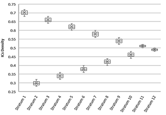
The training dataset contains 24,000 ICs with uniform distribution from ρ=0.3 to ρ=0.7. We arranged ICs in strata of similar density following the structure depicted in Fig. 1. Each stratum has a different density (ρi). If ρi of stratumi is greater than 0.5 is followed by a stratumi+1 of density 1 - ρi. Stratumi+2 has density ρi - 0.04, if ρi is greater than 0.5, otherwise, ρi + 0.04. For each density stratum there are ten bins of 200 ICs, and our GA alternates bins of stratumi and stratumi+1 until the ten bins are consumed for training. In this way we avoid overfitting, and the models are good enough for ICs with majority of 0’s or 1’s indistinctly. Our approach for training is based on iterative learning with alternating strata [23], when after the strata 11 and 12 the GA restart the training with stratum 1.
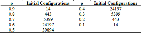
The testing dataset contains 100,000 ICs, according to a Binomial distribution [10], that allows focusing CA evaluation for DCT in the hardest densities. Table 1 shows the density distribution in the testing dataset.
CA identification, on this paper, is achieved through a GA that implements the management of test cases for fitness evaluation, forcing adaptability by iterative changes of the ICs density. In the following section, we describe details of our GA.
2.2. Genetic algorithm description
We developed our GA using the framework for CA identification described in [5]. This framework was developed for problems related to protein contact map representation as a CA, but in this research, we were able to extend its use to 2D DCT. The GA uses in each step 200 ICs of similar density for evaluation: the first half is used as a source of patterns for the neighborhood, and the second one tests the identified CA model. A rule for each CA is obtained similarly to pattern mining, where the rules are probabilistic according to frequencies observed in the dataset. We selected the Matthews correlation coefficient as fitness function because thus, we avoid class bias in IC configurations with density far from 0.5. The general description of the GA is the following.
Initial Population: 100 random CA models with random neighborhoods. The chromosome codifies a possible neighborhood of radius 3 (size 49), which means 249 possible neighborhoods (CA models).
Evaluation: Obtain neighborhood patterns’ frequencies for one stratum in the training dataset for the population. Using the Matthews correlation coefficient, evaluate the result of the simulation for another subset of ICs (to avoid over-adjustment).
Test: Continue until reaching a predefined number of iterations.
New population:
Selection: Top 3% of elite individuals in the population are copied without modification to the next population. Tournament of size eight is applied as the selection method.
Crossover: Uniform two points, rate 0.8.
Mutation: Bit inversion, rate 0.02.
Accepting: All new offspring are added to the new population.
Population replacement: The new population replaces the previous one.
Stratum replacement: Change data stratumi for the stratumi+1 in the training dataset.
Loop: Repeat the procedure from Evaluation.
2.3. Genetic algorithm individual
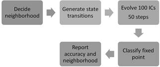
An individual in our GA is a CA with its neighborhood and rule. The chromosome encodes the CA’s neighborhood. We restrict the neighborhood to a maximum local Moore neighborhood of radius 3, so the search space has a size of 249 different CAs. We consider that there is not enough evidence about what is the right neighborhood for DCT, so by deciding a neighborhood we are making a strong assumption about the solution. Despite almost every machine learning approach for 2D DCT selects typical neighborhoods we allow our GA to explore a vast space of neighborhoods, looking for the best solution for DCT. In Fig. 2, we describe the process for evaluation of each CA in the population of the GA. In the first iteration, the GA assigns CA’s neighborhood randomly and after that using recombination and mutation of CAs with the best performance in the previous iteration.
2.4. Baseline models
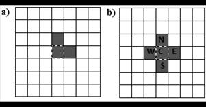
We have chosen two CA models as a starting point of reference. The results for this pair of models allow us to understand some typical characteristics of models that solve DCT. The first one (Toom’s model) is a simple CA that has a small neighborhood (only three cells), and the rule decides the next state by majority vote [15]. Fig. 3.a) shows Toom’s neighborhood, central cell, east cell and north cell. Although this model has low accuracy around the critical density (ρ = 0.5±0.1), for easy test cases the performance is near to perfect (see Table 2).
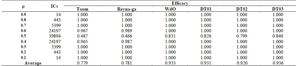
Table 2 Quality measurement for DT01 and benchmark models on the testing dataset.
Source: The authors.
The second baseline model is Reynaga’s CA (see Fig. 3.b). This model’s neighborhood is a restricted version of von Newmann neighborhood but takes only three cells into account, depending on whether the central cell is in state 0 or state 1. The next state is defined by the majority, when central cell state is 0 neighbor cells are C-S-W (central, south, west), in the other case neighbors are C-N-E (central, north, east). Reynaga’s CA performance is almost identical to Toom’s CA, i.e., almost perfect for easy ICs, bad for ρ = 0.5±0.1.
2.5. Benchmark model
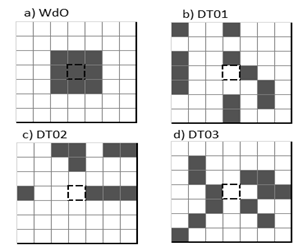
The best model reported by Woltz and de Oliveira [12] is the CA that we are going to use for comparisons. From here on we will call it WdO (according to authors’ last names). WdO was found using an evolutive approach, its neighborhood is Moore radius one (Fig. 4.a), and the rule is standard. WdO is the first ranked model reported in Table 2 in the source paper [12]. The efficacy achieved by WdO in a test of one million ICs, uniformly distributed, was 0.8327, and since its publication was regarded as the best solution for 2D DCT.
3. Results
Cumulative and moving averages are used to measure GA behavior and assessing the stop conditions, since the evaluation function of the best individual is not directly comparable, given that from one generation to another the dataset varies. The high variability originated by the frequent change of training data does not conduce to convergence from a GA iteration but for iteration on the full training set. We describe the best CAs below.
3.1. Best Identified models
The neighborhood of the best CA identified by our GA (named DT01, according to authors’ last names and model version) is shown in Fig. 4.b). A remarkable characteristic of this neighborhood is that the state of the cell to be updated (cell marked with dashes in Fig. 4.b) is not considered to determine its next state: The local dynamics for DT01 depend on the surrounding cells in the neighborhood, but not of the cell itself, which is uncommon in most of the previously proposed models. This kind of topology is a typical machine learning design. DT01 has 2048 rules (11 cells in the neighborhood, 211 patterns), and for all rules majority of states determine the higher probability of transition (more 1s then most probable state 1, 0 otherwise).
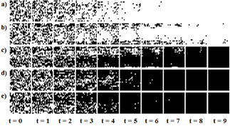
DT01 is a fast converging CA for DCT, i.e., a fixed point is reached in less than 50 simulation steps. Fig. 5 shows examples of fast converging simulations; all the examples converge to a fixed point in less than ten simulation steps.
Source: The Authors.
Figure 5 DT01 application examples on different ICs. Black cells represent estate ‘1’, and white cells state ‘0’. Transitions are shown from left to right. a) ρ0 = 0.43; b) ρ0 = 0.45; c) ρ0 = 0.53; d) ρ0 = 0.54; e) ρ0 = 0.54.
DT02 is a CA that includes nine cells in its neighborhood (Fig. 4.c)) and similarly to DT01, the cell to be updated is not included. This was one of the reasons for which we choose to find out the neighborhood, apparently in our approach the DCT local update depends only on the density around the cell and not in the state of the cell.
DT03 is another one of our best models; its neighborhood contains 12 cells. In our preliminary tests DT03 achieved the best performance. However, we want to make in-depth comparisons between models before drawing conclusions. We describe our assessments in the following sections.
3.2. Quality assessment
We assessed the quality of our models on the testing dataset of 100,000 ICs, and the results are compared with those of Toom’s and Reynaga’s models. In Table 2 we show the efficacies of Toom, Reynaga, WdO and our three models. For each density bin with 0.4 ≤ ρ and ρ ≥ 0.6 the classification is almost perfect. From this fact we can note that for comparisons we just need to consider ICs with ρ close to 0.5 and that the other bins that are in Table 2 can be considered trivial because even simpler models as Toom and Reynaga achieve the best efficacy. DT01 exceeds benchmark models in the average accuracy, being the performance for the three models similar for ρ values over 0.6 and below 0.4. The remarkable difference is observed for the bin of ρ around 0.5, where Toom and Reynaga models show and efficacy close to a random classification. WdO and our three models' performance are similar to the one reported in for WdO [12]. DT03 shows efficacy of 0.84 vs. 0.831 of WdO, maybe someone can conclude that DT03 is the best model, but we believe just a test on a dataset is insufficient to draw conclusions. In the following section we are going to carry on more tests and draw conclusions based on statistical tests.
3.3. Statistical comparison
In machine learning, and specifically in DCT, it is hard to find out statistically significant comparison of approaches. The standard comparison involves the use of a quality measure such as efficacy and several datasets, and the authors draw conclusions about which approach is better than the others based on the maximum count of times that an approach excels the others. The main issue with this style of comparison is that sometimes, the differences are so small that are negligible. In this section we try to draw conclusions about the performance of WdO and our three models using non-parametric statistical tests for multiple comparisons.
We apply the Friedman non-parametric test [24] that computes the average ranking of each model, then test the null hypothesis that all CA perform equally. If the null hypothesis is rejected, then the Friedman test allows us to conclude that the differences in efficacy are statistically significant.
For the analysis in this section, we are going to use five datasets with ρ ∈ (0.5,0.52] ∪ [0.48,0.5) and n × n lattices with n ∈ [21,41,61,81,101]. In each dataset, 10,000 ICs have majority 1s, and 10,000 ICs have majority 0s. The density range grants that we are focusing our analysis exclusively in the hardest cases of DCT. In Table 3 we display the efficacy for each model. If we analyze the efficacy in Table 3 in the typical way the first apparent conclusion is that DT01 excels WdO because the first is the better in three datasets vs. one dataset for the latter. Additionally, the average efficacy is greater for DT01.
In this test, we can note divergence from results in Table 2, where DT03 achieved the best efficacy, but in Table 2, we can see that it is the best just for the dataset of 21 × 21 lattices.
We compare test results using the Friedman non-parametric test, and the Friedman statistic (FF) was 6.84.
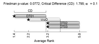
The critical values for FF are: 6.36 at α = 0.1; 7.8 at α = 0.05; 9.96 at α = 0.01. Therefore, we can reject the null hypothesis that all the CAs performed equally at a significance level 0.1. Now, we need to test which CA surpasses with statistical significance, with another. To accomplish this we can use Nemenyi’s post-hoc test described in [24]. Nemenyi’s test defines a critical difference (CD) between the average rankings, and we can conclude that models that overcome the CD have significantly different efficacy. In Fig. 6 we display Nemenyi’s CDs for the four CAs. The bar for each CA indicates its CD and each model that its average ranking does not overlap with others performs significantly better. In Fig. 6, DT01 excels DT02 and DT03, but not WdO. WdO is not significantly better than any other CA because its CD overlaps with all the other models. In conclusion, we can say that at a significance level of 0.1, DT01 is the best CA in our test. However, at higher significance the four tested CAs perform equally.
Source: The Authors.
Figure 6 Nemenyi’s critical difference for efficacy. Stars indicate the average rank of each CA.
What happens if we used different performance measures? We can use the Matthews Correlation Coefficient that is able to capture differences in classifiers that are biased towards one of the classes in the test. For DCT, we have two classes: ICs with majority of 0’s or majority of 1’s. In Table 4, we show the results for the four CAs using the same datasets in Table 3. The direct comparison of scores in Table 4 gives us similar results than for efficacy, but the scores are lowest, showing that there is bias towards the classification of majority of 0’s or 1’s.
Table 3 Efficacy for WdO, DT01, DT02, and DT03 around the critical density ρ=0.5.
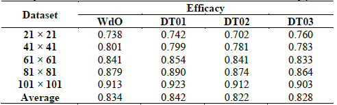
Source: The Authors.
Table 4 Matthews Correlation Coefficient for WdO, DT01, DT02, and DT03 around the critical density ρ=0.5.
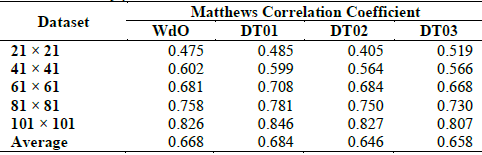
Source: The Authors.
FF for scores in Table 4 was 5.88. The critical values for FF are: 6.36 at α = 0.1; 7.8 at α = 0.05; 9.96 at α = 0.01. In consequence, Friedman's test does not reject the null hypothesis, and we can conclude that there are no statistically significant differences between the four CAs. Although this result is dissimilar to the one we got for efficacy, we conclude there are no significant differences between the compared models.
4. Discussion
We proved that our GA was successful in identifying several CAs that have success similar to the best-known model for 2D DCT. Our reasons for success were three: 1) Our search space is not restricted to a predefined local neighborhood; for 2D DCT there is no evidence about what the appropriate neighborhood is, so we allow that our GA finds out the local neighborhood for each candidate CA. 2) Our training is done by alternating strata that allow our GA to refine the search space covering both classes of ICs and iterating over the training set several times to converge a solution for DCT. 3) We use Matthews Correlation Coefficient to score CAs, so the GA favors those that are less biased.
The maximum neighborhood size for our CAs covers 11.1% of a lattice of size 21 × 21. Though this proportion is large compared the 2% that covers a Moore neighborhood of radius 1, our best CAs just cover 2.5% for DT01, 2% for DT01, and 2.7% for DT03 in a lattice of size 21 × 21. For a lattice of size 101 × 101, our maximum neighborhood size covers just 0.5%, making negligible the impact of the size that we picked. Moreover, as we increase the size of lattice the performance improves (see Tables 3 and 4), so we can say that the size of the neighborhood is not the reason that makes our CAs successful for 2D DCT. In fact, DT02 has the same number of cells as WdO and performed similarly, as was probed by the Friedman non-parametric test.
The typical approach for models’ comparison in DCT and several other machine learning related problems, draws conclusions from direct comparisons of scores. In this research, we find out that this approach lacks statistical significance, and that is needed to draw upon tests that allow to compare multiple models and derive conclusions based on the statistical significance of the results. In our research, our CAs can achieve better results than WdO, but these tests allow us to conclude that our novel CAs perform similarly as WdO on the test datasets.
In our test with a binomial distribution, we notice that ICs with densities over 0.6 and below 0.4 are uninteresting because the tested models can perform correctly in this range. So, is necessary that researchers exclude this range in analysis to get a precise measure of the performance of the CA. It is better to restrict the range of densities in the interval [0.48, 0.52] so that comparisons allow us to determine when a novel CA for DCT is better at the critical density.
We used Matthews Correlation Coefficient as an alternative performance score for DCT. With it, we can improve performance assessment because we can obtain a measurement of bias in our classifications. Efficacy assesses the proportion of correct classified ICs, while Matthews Correlation Coefficient decreases when a class has bias in the proportion of correctly predicted ICs. We suggest that an analysis that uses both measures can give a better assessment of the real performance of CAs in DCT. Additionally, we used Matthews Correlation Coefficient as score for CAs in our GA, so we prefer models that are more balanced in DCT classification.
5. Conclusion
Our approach successfully identifies CA models for DCT, not just improving efficacy, but also showing adequacy and usefulness of the architectural framework used. Although our identified CA models provide remarkable results in DCT, our framework’s methodological success is an important aspect that opens the door for new research topics. We already are developing a novel approach for contact map prediction based on CA identification framework used for DCT.
Our main goal was to test our architectural framework [5] for CA identification. The framework provides design patterns for the implementation of metaheuristics and predefined services that are extensible and useful for CA model identification. Here we show how the framework worked for 2D DCT. Upon the results of this work, we are working on the topic of CA model identification for protein contact map prediction.

