


 Inglês (pdf)
 Artigo em XML
 Referências do artigo
 Enviar este artigo por email
 Citado por SciELO
  Citado por Google
  Similares em
SciELO
Similares em
SciELO  Similares em Google
 Permalink
1. Introduction
Recently, several quantum devices, with up to tens of qubits on universal quantum computers (UQC) and thousand qubits on annealer (QA) devices, have become available through the cloud. This enables the possibility to use real quantum hardware to solve very simple problems for first time. However, in the near term, those devices are expected to be very limited in number and quality of qubits. These quantum computers represent prototypes that are not scalable and sufficient to test complex quantum algorithms. The construction of a full-scale quantum computer comprising millions of qubits is a longer-term prospect. Quantum computer prototypes are currently very small and specific and are not yet able to overcome the processing capacity of classical computers. For example, the recent IBM Q System One [1] only operates with 53 qubits. Programming this prototype still lacks the compiler support that modern programming languages enjoy today. Programmers of this machine must design low-level circuits; they must map logical qubits into physical qubits that need to obey connectivity constraints. This task resembles the early days of programming, in which software was built in machine languages [2].
For all this, quantum computing simulators are the only widely available tools to design and test quantum algorithms. However, the simulation of quantum computing models in classical computers requires exponential time and involves extremely complex memory management. The problem is that using conventional techniques to simulate an arbitrary quantum process that is significantly larger than any of the existing quantum prototypes would soon require a huge amount of memory on a classical computer. For instance, to simulate a 60 qubits quantum state the process would take about 18.000 petabytes (18 Exabytes) of classical computer memory. Therefore, researchers try to reduce such challenges by proposing efficient simulators. Some popular quantum software simulators can be found in [3,4].
The simulation of quantum systems in classical computers is a relatively old problem. However, with the emergence of real quantum computers, the limit of what classical simulations can handle is being pushed to better understand its operation and verify that t is behaving as predicted. The simulations of NISQ (Noisy Intermediate-Scale Quantum) devices on classical computers represent an invaluable experimental testbed for noise characterizations, for the development of quantum error correction, and for the verification of quantum systems. With this momentum, a variety of techniques have been invented to keep up with the newer quantum processors [5].
This work attends to address the fundamental details of quantum simulation on classical computers and the problems related to it. We use a useful quantum algorithm and its implementation on two popular quantum simulators to illustrate these aspects.
2. Key concepts of quantum computing
To better understand the quantum computing model, it is necessary to know the key aspects of the inheritance of quantum mechanics and the fundamental concepts on which quantum computing is based.
2.1 Qubit
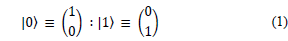
A physical qubit Is a physical device that behaves as a two-level quantum system. A logical qubit is a unitary vector in a two-dimensional Hilbert space in which the Boolean states 0 and 1 are represented by a prescribed pair of normalized and mutually orthogonal quantum states denoted using Dirac’s notation |0〉 and |1〉 [6].The two states form a “computational basis”, and any other (pure) state of the qubit can be written as a superposition α|0〉 + β|1 [7].
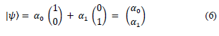
The state |ψ〉 associated with a qubit can be any unit vector in the two-dimensional vector space spanned by |0〉 and |1〉 over the complex numbers [8]. The general state of a qubit is:
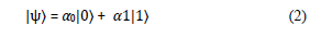
Where α0 and α1, are called the amplitude of component |0〉 and component |1〉 respectively, are two complex numbers constrained only by the requirement that |ψ〉, like |0〉 and |1〉, should be a unit vector in the complex vector space, in other words, only by the normalization condition: |α0|2+|α1|2 = 1. The state of n qubits is spanned by the tensor product basis.
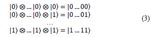
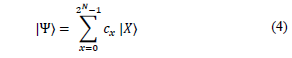
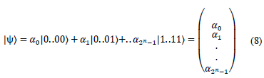
The general equation of a n-qubit state is
2.2 Superposition
The special characteristic of quantum states is that they allow the system to be in a few states simultaneously, this is called superposition. Quantum bits are not constrained to be wholly 0 or wholly 1 at a given instant. In quantum physics, if a quantum system can be found to be in one of a discrete set of states, which we’ll write as |0〉 or |1〉, then, whenever it is not being observed it may also exist in a superposition, or blend of those states simultaneously [9].
2.3 Measurement of single qubit quantum state
According to the postulate 3 of quantum mechanics (Measurement), the action of measure a quantum state produces a change in it. If a state |v〉= α|0〉 + β|1〉 is measured and the outcome is |0〉, then the state |v〉 changes to |0〉. A second measurement with respect to the same basis will return |0〉 with probability 1. To understand this, it is necessary to think of a superposition |v〉 as a state that could be in both state |0〉 and state |1〉 at the same time, that is to say, the quantum state |v〉 is a combination of |0〉 and |1〉 in similar proportions but with different amplitudes. A fundamental fact about this measurement process (measurement in the computational basis) is that the quantum state |v〉 v is disturbed by the measurement. Therefore, it is impossible to determine the original state from any sequence of measurements [10].
2.4 Entanglement
The “entanglement” describes a correlation between different parts of a quantum system that surpasses anything that is classically possible. It happens when the subsystems interact in such a way that the resulting state of the whole system cannot be expressed as the direct product of the states of its individual parts. When a quantum system is in such a tangled state, the actions performed in one subsystem will have a side effect in another subsystem, even if it does not act directly on that subsystem [9]. It takes 2n - 1 complex numbers to describe states of an n-qubit system. Because 2n is much bigger than n, most of the n-qubit states cannot be described in terms of the state of n separate single-qubit systems. States that cannot be written as the tensor product of n single-qubit states are called entangled states. Thus, the vast majority of quantum states are entangled [10]. If we can write the tensor product of those states, they are said to be separate states.
2.6 Reversibility
The reversibility is a property of some operations that consist of obtaining unique inputs for all outputs of said operations. Reversibility is one of the most useful mechanisms in quantum computing. Reversible operations change the initial state of the qubits into its final form using only processes whose action can be inverted. There is only a single irreversible component to the operation of a quantum computer, the measurement, which is the only way to extract useful information from the qubits after their state has acquired its final form [8]. In a reversible operation, every final state arises from a unique initial state.
2.7 Decoherence
Quantum states are very fragile and susceptible to noise. Eventually, errors inevitably appear over time, this process is known as decoherence. Some situations that cause errors are, for example, atoms couple to the electromagnetic field and spins couple to other spins via dipole interactions. These unwanted couplings cause errors; therefore, quantum states must be well isolated from the environment in order to protect quantum information against these errors.
In the context of quantum computing, qubits are susceptible to more kinds of errors than are classical bits. There are phase errors that send |0〉 → |0〉 and |1〉 → -|1〉, which has the effect of changing α|0〉 + β|1〉 to α|0〉 - β|1〉. In addition, there are generally small errors that have the effect α|0〉 + β|1〉 → (α+O(ϵ)) │0〉 + (β+O(ϵ)) |1〉 where ϵ≪1 is a parameter that characterizes the size of the error. It is necessary to take special care in detecting an error because measuring a state can change it, and of course, we cannot just copy the qubit state, because of the no-cloning theorem [6].
2.7 Quantum computing models
A quantum computing model is the description of the different scientific approaches to formalizing the transformations over inputs to compute outputs using quantum resources. A model is determined by the basic elements in which the computation is decomposed [11,12]. The four main models of practical importance are:
Quantum Gate Array or Quantum Circuit: The computation is decomposed into a sequence of few qubit quantum gates.
One-way quantum computer: The computation is decomposed into a sequence of one-qubit measurements applied to a highly entangled initial state or cluster state.
Adiabatic quantum computer: The computation is decomposed into a slow continuous transformation of an initial Hamiltonian into a final Hamiltonian, whose ground states contain the solution.
Topological quantum computer: The computation is decomposed into the braiding of anyons in a 2D lattice.
3. Basis of quantum computing simulation
In classical computing, the amount of information contained by a specific state using n bits is n, there will be only one combination of n 0s and 1s. In quantum computing, a state composed of n qubits will be a union of all possible combinations of n 0s and 1s. That is to say, the size of the information is 2n. For example, if we are using 3 bits, we will have just one of the 23 possibilities whose length is 3, for instance, 010. If we use 3 qubits we will have, not only one but all combinations: 001, 010, 011. 111, each one multiplied by the corresponding amplitude. If we increase in 1 the number of bits the size will be n + 1, but if we increase the number of qubits, we get the double of the size, that is to say, 2n+1 [13].
3.1 Single Qubit representation
A qubit is a two-level quantum system. The state |ψ〉 of this quantum system can be represented by two complex numbers α0 and α1 such as

When we measure the qubit, we obtain |0〉 with probability p= |a0 |^2 or |1〉 with probability 1-p= |a1 |^2. Thus, after being measured, the qubit becomes a classical bit. To store |ψ〉 on a classical computer, it is more suitable to use two orthonormal vectors to represent |0〉 and |1〉.
3.2 Operations on single Qubits
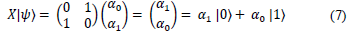
Any operation on the qubit of eq. (7) is represented by a complex unitary matrix. For example, if we apply a NOT gate (X gate), it is equivalent to execute a matrix-vector multiplication.
3.3 n-Qubits representation
In a general form, the n-qubits state of a quantum computer can be represented by a complex vector of size 2 n .
3.4 Operations on n-Qubits
The operations on the state of eq. (8) are 2n×2n unitary matrices. Finally, applying a single-qubit gate U to the i-th qubit of an n-qubit quantum computer amounts to multiplying the state vector of coefficients αi by the matrix.
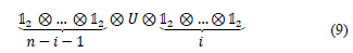
This is a complex sparse matrix-vector multiplication of dimension 2n. Therefore, for double-precision values, just storing the state vector for 50 qubits would already require 16 petabytes of memory.
3.6 Quantum state preparation
Patrick Coles et. al. in his work [14] presents some methods to prepare qubits states. The preparation procedure of an n- qubit state consists of two steps:
Finding a unitary transformation that takes the N-dimensional vector (1, 0, . . . 0) to the desired state (α1, ..., αN), where N = 2n.
Rendering the unitary transformation into a sequence of gates.
To briefly exemplify this procedure, let us see how to prepare a single qubit state |ψ〉 It is represented as a superposition of 0 and 1 states |ψ〉= α|0〉+ β|1〉 where |α|2+|β|2=1. The magnitudes |α|2 and |β|2 represent the relative probability of |ψ〉 being 0 or 1. Until a non-observable global phase, we can assume that α is real, so that |ψ〉= cosθ|0〉+ eiϕ sinθ|1〉 for some angles θ, φ. Therefore, we represent the state as a point on the unit sphere with θ the latitude and φ the longitude. Thus, one qubit state preparation consists simply of finding the unitary transformation that takes the north pole to (α, β). To set the initial state of more than one qubit we can use the so-called Schmidt decomposition. It allows one to initialize a 2n-qubit state by initializing a single n-qubit state, along with two specific n-qubit gates, combined with n CNOT gates.
4. Quantum algorithms
A quantum algorithm is an algorithm made in one of the models of quantum computing, with quantum circuits as the most used model. A classical (or non-quantum) algorithm is a finite sequence of instructions, or a step-by-step procedure for solving a problem, where each step or instruction can be performed on a classical computer. Similarly, a quantum algorithm is a step-by-step procedure, where each of the steps can be performed on a quantum computer. Although all classical algorithms can also be performed on a quantum computer, the term quantum algorithm is generally used for those algorithms that incorporate some essential features of quantum computing, such as superposition or entanglement [11]. The field of quantum algorithms has become a sufficiently large area of study “Quantum Algorithms Zoo” [15] cite almost 400 articles in this area.
When referring to an algorithm, the computational complexity, or just complexity, is a measure of the resources used by the algorithm, usually measured as a function of the input size of the algorithm. The complexity for the input size n is taken as the cost of the algorithm in a more unfavorable case entry for the size n problem. When referring to a problem, the complexity is the minimum amount of resources required by any algorithm to solve the problem [16]. In the theory of computational complexity, asymptotic scales of complexity measures such as execution time or problem size are generally considered. In both classical and quantum computing, the execution time is measured by the number of elementary operations used by an algorithm. In the case of quantum computing, this can be measured using the quantum circuit model, where a quantum circuit is a sequence of quantum operations called quantum gates, each applied to a small number of qubits. To compare the performance of the algorithms, the notation O(f(n)) of the computing style is used, which is interpreted as “asymptotically delimited by f (n)” [17]. In these cases, it is convenient to use the basic ideas of the theory of computational complexity [18], especially the notion of complexity classes, which are groupings of problems by difficulty. The informal descriptions of some important complexity classes are.
Class P: A deterministic classical computer can solve it in polynomial time.
Class BPP: A probabilistic classical computer can solve it in polynomial time.
Class BQP: A quantum computer can solve it in polynomial time.
Class NP: A deterministic classical computer can check the solution in polynomial time.
Class Quantum Merlin-Arthur: A quantum computer can check the solution in polynomial time.
If a problem is said to be complete for a complexity class, this means that it is one of the “most difficult” problems within that class [17].
There are three classes of quantum algorithms with clear advantages over known classical algorithms.
Algorithms based upon quantum versions of the Fourier transform, which is very used in classical algorithms.
Quantum search algorithms.
Quantum simulation. A quantum computer is used to simulate a quantum system.
4.1 Quantum parallelism
One of the main features of quantum computing is to take advantages of quantum mechanics effects like superposition and entanglement, to speed up the calculations. In 1985 Deutsch [19] found a computational problem that could be solved on a quantum computer in a manner that is impossible classically. In 1992 Deutsch and Jozsa [20] simplified and extended the earlier result.
4.2 Quantum algorithms workflow
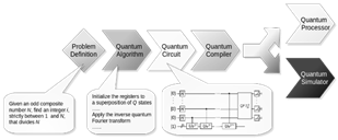
A typical quantum algorithm workflow on a gate-model quantum computer is depicted in Fig. 1. It begins with a high-level definition of the problem, for example, Shor’s algorithm. The problem to solve is, given an odd composite number N, we need to find an integer i, strictly between 1 and N, that divides N.
5. Quantum computing simulators
A quantum simulator is an object able to execute quantum computations. They can be classified in two categories [21]:
A Quantum System that can perform very specific quantum computations.
Software Packages that can reproduce most of the fundamental aspects of a general universal quantum computer on a general-purpose classical computer.
Real quantum computers are available to use over the cloud, however, they are still very small to be considered as a complete universal quantum computer. On the other hand, although quantum computing simulators, running on a classical computer, cannot process actual quantum states they are very helpful to test the code syntax and flow.
There has been a recent explosion of quantum software platforms which can overwhelm to those looking for a platform to use. Therefore, this section attempts to mention some of the most popular initiatives.
5.1 Popular open-source quantum computing simulators
Many institutions are working on quantum software, specifically quantum simulators, from academic research groups to big companies. A list of the very recent developments is maintained in several websites [3,4,22,23]. They present several quantum computing software packages developed by different organizations. LaRose et. al. [24] made a review of some important general-purpose projects, that operate at the level of quantum gates. Guzik [25] did a study on the appropriate approach to implement different models of quantum computing. Fingerhuth et. al. [26] did an evaluation of a wide range of open source software for quantum computing, including all stages of the quantum toolchain from quantum hardware interfaces through quantum compilers to implementations of quantum algorithms, as well as several quantum computing models: quantum annealing and discrete and continuous-variable gate- model. The criteria used by this team to select the projects involve aspects like approved license, maturity, number of contributors, repository availability, etc.
Leveraging all those works, we present the following list with a specific selection of major software quantum simulators developments:
Quantum++ (C++) Is a general-purpose multi-threaded quantum simulator written in C++ with high performance [27].
QuEST (C/C++) It is an open-source quantum simulator with multithreading, distributed processes and GPU- accelerated capabilities [28].
Qrack (C++) Is a quantum simulator written in C++ that comes with additional support for Graphics Processing Units (GPUs) [29].
Intel-QS Formely qHiPSTER, is a simulator of quantum circuits optimized to take maximum advantage of multi- core and multi-nodes architectures [30].
Some projects provide a full-stack approach to quantum computing, including not only a simulator but compilers and the possibility to run the program on real quantum processors. The following list shows some of these projects:
XACC, Simulator: TNQVM (C) This provides an implementation that takes advantage of the tensor network theory to simulate quantum circuits [31,32].
Qiskit, Simulator: Qiskit Aer (Python) Framework for working with noisy quantum computers at the level of pulses, circuits, and algorithms supported by IBM [33,34].
ProjectQ, Simulator: ProjectQ (C++, Python) An open source software framework for quantum computing [35,36] supported by ETH Zurich.
Forest, Simulator: QVM (Python) Is the quantum simulator of the full-stack library Forest. It is a purely Python- based simulator which is meant for rapid prototyping of quantum circuits. It is supported by Rigetti.
6. Quantum simulations resource usage
To illustrate the resources consumption by a quantum simulator, we run the Fourier Quantum Transform (QFT) using two quantum simulators. Before present the results of the simulations we describe in the next subsection the details of the QFT algorithm.
6.1 The Quantum Fourier Transform
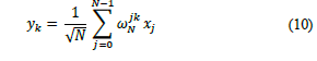
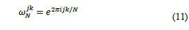
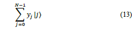
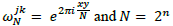
Quantum Fourier Transform (QFT) is a quantum implementation of the discreet Fourier transform [37]. The quantum Fourier transformation is a generalization of the Hadamard transformation. The difference is that QFT introduces phase. The specific types of phases introduced by QFT are the primitive roots of the unit, ω. Let’s remind that in the complex numbers, the equation zn=1 has n solutions, for example: for n = 2 z could be 1 or-1, for n = 4 z could be 1, i, -1 or -i. These roots can be written as power of ω= 22πi/n. This number ω is called a primitive nth root of unity. DFT is a transformation of a set x0, ...xN−1 of N complex numbers into a set of complex numbers y0, ...yN−1 defined by eq. (10).
Where
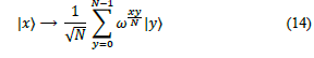
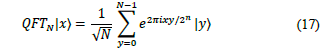
To build the quantum version of DFT let’s define a linear transformation U on n qubits that acts on computational basis states |j〉 where 0≤j ≤ 2n-1. In other words, QFT acts on a quantum state like
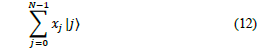
And map it to the following quantum state.
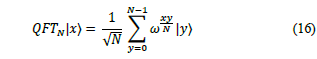
That transformation is performed using the formula of eq. (10). If we consider it action on superpositions we note that it corresponds to a vector notation for the Fourier transform for the case N= 2n. Considering the action of QFT on an orthonormal basis |0〉,…,|N-1〉, we can define it as a linear operator with the following transformation on the basis states.
That action on an arbitrary state can be written as
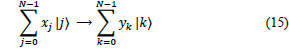
Where the amplitudes y k are the discrete Fourier transform of the amplitudes xk. It can be checked that this transformation is a unitary transformation, and thus can be implemented as a quantum circuit.
6.1.1 N-Qubits QFT
This section describes the QFT for N Qubits. Simple examples for one and three qubits can be consulted in [34]. The following operations have to be performed to obtain the quantum Fourier transform for N qubits.
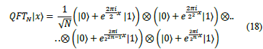
Since
Rewriting in fractional binary notation, expanding the exponential of a sum to a product of exponentials, rearranging the sum and products, and expanding again
6.1.2 QFT quantum circuit
The circuit that implements QFT uses two quantum gates: The Hadamard gate and two qubits-controlled rotation gate CROT k . The last is represented by the following matrix.

Where
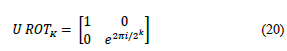
The gate UROT k is the phase gate with the following matrix representation. Fig. 2 shows the n-qubits quantum circuit for QFT.
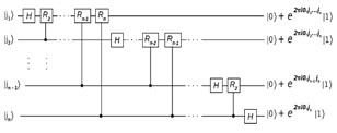
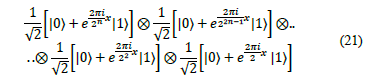
The circuit of the Fig. 2 operates as follow: starts with n-qubit input state, |x 1 ,x 2 ,..,x n 〉. Apply the H gate on qubit 1. Then, apply the CROT2 gate on qubit 1 controlled by qubit 2. After that, apply the CROT3 gate on qubit 1 controlled by qubit 3. Then, apply the CROTn gate on qubit 1 controlled by qubit n. Finally, apply the similar sequence of gates on qubit 2 to qubit n. The final state is.
In terms of performance, DFT takes N log N=n2n steps to transform N=n2n numbers. On a quantum computer, the transform can be accomplished using log2N=n2n. It seems that quantum computers can be used to very quickly calculate the Fourier transform of a vector of 2n complex numbers. However, the Fourier transformation is performed on the “hidden” information in the amplitudes of the quantum state.
This information is not directly accessible in the measurement process. The problem, of course, is that if the output status is measured, each qubit will collapse in the state |0〉 or |1〉, preventing us from learning the result of the transformation yk directly.
7. Results
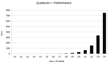
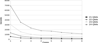
Among the big list of software quantum simulators available in [3,4,23] we have chosen Quantum++ and Intel-QS. Quantum++ was selected for its simplicity of operation and open-source code. Also, it provides a benchmark for QFT and the ability of parallel execution on a single node. Intel-QS was selected because it uses the parallel studio to optimize the code and the MKL library to increase the performance, also this simulator is open source and provides a QFT implementation. The experiments were performed using a range of 10 to 24 qubits to obtain a proper scale to observe the results. Simulations under 10 qubits take a fraction of a second and do not provide important contributions to the analysis. The hardware used was a laptop with an Intel i7-8565U 1.8 GHz processor and 16 GB of RAM. The first experiment was performed using Quantum++ simulator using OpenMP parallelization. We fix the number of threads in 8 to leverage the total power of the processor and varied the number of qubits from 10 to 24. A shell script was used to automate the execution procedure. Build instructions and the QFT source code corresponding to the quantum circuit illustrated in Fig. 3 can be found in [38]. Fig. 4 depicts the performance of Quantum++ simulator.
To show how performance is improved when we increase the number of threads, we run an experiment using the Quantum ++ simulator by varying the number of threads from 1 to 8. To correctly observe the results, we use a range of 21 to 24 qubits since for a lower number of qubits, the simulation requires a small amount of time and we cannot see the speedup, and for a higher number of qubits, the simulation exceeds the hardware capacity. Fig. 6 depicts these results.
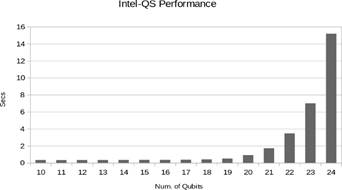
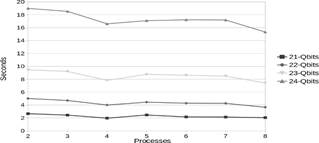
The next experiment was performed using Intel-QS simulator using MPI with 8 processes. Fig. 5 depicts the results.
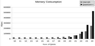
In the same way, we simulate QFT using Intel- QS for a range of 21 to 24 qubits, this time using a MPI approach when varying the number of processes from 2 to 8. Fig. 7 depicts the memory usage vs the number of qubits. Here, we compare both simulators.
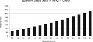
Finally, in Fig. 8 we can observe the total number of gates used in the quantum circuit of QFT for different number of qubits.
8. Discussion
Analyzing the results depicted in Figs. 3 and 4 we notice that Intel-QS has a significantly better performance than Quantum++, in terms of processor usage. In Fig. 5 we note that increasing the number of threads the execution time improves substantially. The execution time for 24 qubits using one thread was 6912.03 seconds and using 8 threads was 1158.79 seconds. Thus, we obtained a good speedup. Conversely, Fig. 6 shows that Intel-QS shows less acceleration than Quantum++ and in some cases there is no acceleration at all. In Fig. 7 we observe that for small number of qubits Quantum++ has a better memory management, however, Intel-QS is better for more than 22 qubits. We can notice that memory usage is substantially big after 21 qubits and, in general, as we increase one qubit the memory usage is approximately double. If we follow that trend, we can infer that for 30 qubits we will need 32 GB of RAM and for 45 qubits one Petabyte of RAM. In addition, we notice that Intel-QS has a better memory management. Observing Fig. 8 we can note that the total number of gates of the QFT quantum circuit increase approximately linearly with the number of qubits. Finally, it is clear that Intel-QS can scale better than Quantum ++ due to its distributed nature which allows it to use more resources if we run it in an HPC cluster.
9. Conclusions
Quantum computing simulators, running on a classical computer, cannot process actual quantum states, however, they are very helpful to test the code syntax and flow. Although some of them can simulate decoherence, an important feature of quantum simulators is that they can simulate quantum states without errors, which allows us to concentrate on the details of the algorithms and their operation. Despite these important advantages, quantum simulators consume a huge amount of classical resources as we can observe in the results section, being the memory the most critical issue, for example, the amount of RAM memory needed to simulate a quantum circuit representing the quantum Fourier transform algorithm for 45 qubits is approximately one Petabyte. Therefore, it is imperative to design quantum simulators using novel techniques to test quantum algorithms with useful dimensions. It must be pointed out that HPC is a fundamental tool to build this type of simulators to handle quantum algorithms with proper dimensions to get useful outcomes.
The next steps could include the use of a supercomputer to scale the experiments carried out in this work and include other simulators to extend the comparison process. On the other hand, several initiatives are trying to reduce the consumption of classical resources by quantum simulators, for example, Jianxin Chen et. al. [5] works on a new technique, based on Google’s model for variable elimination in the line graph, that implement a single-amplitude simulator, Aidan Dang et. al. [39] studies how the entanglement structure of Shor’s algorithm [40] is suitable for a particular matrix product state representation, that quantifiably reduces the computational requirements for simulating it in a classical computer and Xin-Chuan Wu et. al. [41] implements a lossy compression algorithm to reduce the amount of memory usage. The aim is to re-design quantum simulators using at least one of these techniques, or a mix of them, to test quantum algorithms with useful dimensions.
One of the main problems with software quantum simulators is that they demand a huge amount of resources, specifically, RAM memory. Different research teams have been working on the implementation of advanced techniques to overcome this issue. For example, the use of procedures to make the operations with quantum gates instead of representing them as traditional data structures. It allows saving memory space but involves an increment in the processing time. The vector space compression could also result in a processing overhead. Therefore, there is not any standard approach to deal with the resource consumption by the software quantum simulators.

