


 English (pdf)
 Article in xml format
 Article references
 Send this article by e-mail
 Cited by SciELO
  Cited by Google
  Similars in
SciELO
Similars in
SciELO  Similars in Google
 Permalink
1. Introduction
Type 2 sedimentation is a process whereby particles agglutinate as they settle [1]. However, determining the removal efficiency of this type of particles in a settler is a complex process since the particles that are generated change their shape and size, affecting the sedimentation rate [2].
Traditionally, the determination of the percentage of removal of flocculent particles is carried out from a graphic method, by means of which isoconcentration curves are constructed that relate the values of the percentage of removal obtained from the sedimentation column, associated with time and depth at which the sample is taken [3]. This method has been adapted and modified by different authors, until a graphical integration methodology is obtained, which contemplates the experimental data to calculate the total removal [4]. If it is taken into account that the construction of isoconcentration curves is a tedious, inaccurate process, susceptible to human error and that it may have problems when reproducing them [5], different authors have developed mathematical equations in order to eliminate these problems: [6-10], and others have used two-dimensions transport models and computational fluid dynamics (CFD) for simulate the settling process and improve tank efficiency [11-13].
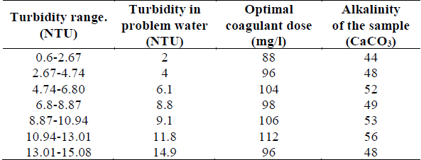
Previous studies on this topic, coincide in using for their experiments, initial turbidity values in the problem water above 100 NTU [4,5,10-12]. Turbidity values in these ranges are characteristic of waters with medium and high levels of turbidity. However, there is a need to evaluate the accuracy of at least one of the previously developed mathematical equations, when the initial turbidity in the test water is low.
In this article, the determination coefficient R2 is calculated to evaluate the goodness of fit of the San model in the calculation of the percentage of removal of flocculent particles, when the initial turbidity in the problem water is low (characteristics of mountain rivers). For this, a frequency analysis of the historical turbidity data that enters four drinking water treatment plants located in the department of Cundinamarca (Colombia) is made, in order to establish what are the typical values that enter said plants. By means of a jar test, the optimal doses of aluminum sulfate for each sample are defined and the remaining turbidity is measured in a sedimentation tower that allows determining the percentage of removal of particles as a function of the sedimentation time and the depth of the sedimentation. tower.
The results obtained show that for initial turbidity in the test water lower than 11.8 NTU, the San model presents certain limitations in determining the percentage of removal of flocculent particles, evidencing the existence of a restriction in the use of said equation.
2. Materials and method
The development of this study begins with an analysis of the frequency distribution of the turbidity of the raw water that enters 4 drinking water treatment plants (PTAP) located in the department of Cundinamarca, in order to establish the characteristic ranges of turbidity that enters these plants. With the turbidity ranges already established, a test water is prepared in the laboratory whose nephelometric turbidity units (NTU) are within the turbidity limits defined in the frequency distribution analysis.
Using a jar test, the optimal dose of coagulant to be added is defined for the 7 samples of the test water prepared in the laboratory. Alkalinity and pH are also measured for each sample, evaluating that the latter presents a value close to neutral, in such a way as to minimize the effects of pH variation in subsequent processes.
Next, each water sample is subjected to a coagulation-flocculation-sedimentation process in a sedimentation tower and the remaining turbidity is finally measured at different time intervals and different depths.
With the measured data, a multiple linear regression is made, by means of which a potential equation is fitted to the data series that relates the percentage of removal of the flocculent particles, with time and depth of sedimentation.
2.1 Turbidity ranges analyzed
The input information to define the ranges of turbidity to be used in the present study was extracted from the platform of the single home public services information system (SUI). In this case, 4 water treatment plants located in the department of Cundinamarca were chosen: a Drinking Water Treatment Plant (DWTP) located in the city of Bogotá and the DWTPs of the municipalities of Facatativá, Madrid and Chipaque.
The frequency analysis of the historical data was carried out using the methodology presented by [16], following the procedure described below.
A. Rank It is the numerical variation of the variable; it is the path that the variable takes from the smallest value to the highest value.
The range is calculated as the difference between the highest and the lowest value in the sample as shown in Equation (1).
B. Number of intervals or classes.
The number of intervals is defined from the total number of data in the sample, using Equation (2).

The number of turbidity data obtained from the SUI platform was 2056. This value corresponds to the total amount of turbidity values recorded at the entrance to the 4 plants.
C. Amplitude or class interval
The amplitude determines the extension that each of the previously determined ranges will have. This parameter is calculated as the relationship between the range and the number of intervals as shown in Equation (3).
D. Limits of the intervals.
When constructing the intervals, each of them is determined by two extremes: lower limit (Li) and upper limit (Ls). For the first interval, the lower limit is equal to the lower limit of the range Li and the upper limit of this interval is formed by adding the amplitude (C) to the lower limit. The second interval starts from the upper limit of the first interval and the amplitude is added to obtain the upper limit. This process is repeated for the total of intervals in which the data set was grouped.
E. Absolute frecuency
The absolute frequency (ni) is the number of times the value (Xi) of the variable X occurs in the sample or population.
2.2 Preparation of the test water
The preparation of the test water was carried out by adding bentonite to one liter of drinking water until obtaining a turbidity of the water within the ranges obtained from the frequency analysis of the historical data. The process consists of weighing the bentonite, then diluting it in a liter of water and then using a turbidimeter to take the final turbidity reading of the sample.
The first two turbidity levels for the preparation of the test water were obtained by trial and error. With these two initial values, a linear regression was performed and an equation was obtained that relates the amount of bentonite to be applied with the desired turbidity and that also allows to calculate the dose of bentonite for the other samples.

In Equation (4), CB is the amount of bentonite to add and T is the final turbidity of the water.
2.3 Jar test - determination of mixing parameters
Coagulation is carried out using type A aluminum sulphate. The optimal dose of the coagulant is determined by a jar test, taking into account the initial turbidity of the test water and following the methodology presented by [17]. Table 1 shows the optimal dose of coagulant according to the turbidity of the water.
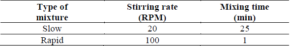
The stirring speeds and mixing time reported by [18] were defined for fast mixing and for slow mixing. The values used are shown in Table 2.
2.4 Sedimentation test
In the same sedimentation tower, the coagulation, flocculation and sedimentation processes are carried out. Rapid mixing is done by adding compressed air through the lower part of the tower at a pressure of 30 psi and for a time of 1 minute, for slow mixing the air pressure is reduced to 5 psi for a time of 25 minutes.
Once the mixing process is finished, the air supply to the system is interrupted and it is left at rest measuring the remaining turbidity at different time intervals and for different depths.
The above procedure is repeated for each of the turbidity ranges obtained from the frequency analysis of historical data, as shown in Table 1.
2.5 Calculation of the percentage of particle removal.
With the remaining turbidity measured in the sedimentation tower, the percentage of removal of the particles (as a function of turbidity) is calculated as a function of the sedimentation time and the depth of the tower. The results obtained are shown between Figs. 2 and 8.
The initial data of the remaining turbidity in the tower was measured 5 minutes after the system was at rest, subsequently data was taken every 10 minutes.
2.6 Statistical adjustment by multiple linear regression.
There are different studies on curve fitting to calculate the percentage of particle removal or settling velocity in sedimentation process. For example, in hindered settling the mathematical relation between the sludge concentration and the zone settling velocity can be described by an exponential decaying function [19-21]. In the other hand, for flocculent particles, different authors have reported studies about empirical equations for calculating velocity and the percentage of removal of flocculent particles) in a sedimentation tower.
In the first case: [10] present an integrated velocity form to estimate flocculent settling velocity of fine suspend particles, the proposed velocity models offer an advantage over other interpolated-isopercentile models which are prone to numerical errors during interpolation. [22] present a simple approach for estimating the flocculent settling velocity of fine suspended particles, the empirical flocculating equation is expressed as a function of time, depth and others constants.
In the second case: [7] developed an empirical equation for iso-percentage suspended solids removal curves obtained from sedimentation tests and uses empirical parameters in the equation to calculate overall suspended solids removal efficiently in a sedimentation basin. [6] fitted a simple approximating function to quiescent settling test data is given that can serve for either discrete or flocculant settling. The method is illustrated using concentration data and the results are compared with values calculated by the traditional method. Ozer [8] proposed an exponential equation as a function of time, depth and other parameters associated with the regression curve for calculate the velocity settling and concentration percentage of sediment.
The present study is carried out using San's equation due to its mathematical simplicity and consistency.
Where a, b and k are the specific parameters of a given suspension, P is the percentage of material removed, T is sedimentation time, and H is the depth in the sedimentation tower. From the Iso-concentration curves and by means of a multiple linear regression. The constants a, b and k presented in Equation (5) are calculated.
3. Results and discussion
3.1 Typical turbidity entering the analyzed plants
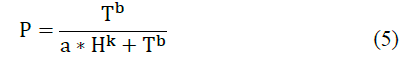
Fig. 1 shows the results of the frequency analysis of the historical turbidity data, which enter the four plants selected in the present study. The trend of the data, in these plants, follows an asymptotic behavior towards the ordinate axis, showing that, for the most part, the turbidity that enters these plants is low.
Of the historical data analyzed, 76% of the time the turbidity is less than 6.4 NTUs, 12.5% is between 6.4 - 12.2 NTUs, 5.8% is between 12.2 - 15.5 and the remaining 5.7% the turbidity is greater than 15.5 NTUs. The minimum turbidity value recorded is 0.6 NTUs and the maximum value is 70 NTUs. These results may be due to the location of the surface water catchment sources, which are in the upper parts of the basins and / or to the fact that the parameter measurements were carried out during summer periods. However, the SUI platform does not mention the environmental conditions present at the time the sample was taken.
Source: The authors.
Figure 1 Frequency analysis of historical turbidity data entering the four plants
Taking into account that about 94% of the data is between 0.6 NTU and 15.5 NTU, turbidity values higher than 15.5 NTU were not taken into account for the study and the frequency analysis was performed again, obtaining the ranges and values of initial turbidity presented in Table 1.
Table 3 shows the initial turbidity ranges used in previous studies to determine the percentage of removal of flocculent particles in type 2 settlers. The initial turbidity in the reference studies vary from a minimum value of 100 NTU to a maximum value of 1000 UNT.
When comparing the initial turbidity values used in the present study (less than 15 NTU), with the initial turbidity values reported in reference studies, it is clear that, in the latter, the analysis focuses on turbidity values that we could classify as high (above 100 NTU). Low turbidity values present a high probability of occurrence (see Fig. 1), especially in the upper parts of the basins, where the concentration of dissolved solids in the water is low, since there are not large contributions of polluting loads to cause by anthropogenic activities and / or soil erosion.

3.2 Percentage of removal of flocculent particles
From Fig. 2 - 8 shows the results of percentage removal of flocculent particles in the water column, for each of the initial turbidity in the test water. The behavior of the iso-percentile lines is characteristic of type 2 sedimentation, where for the same removal efficiency, the relationship between time and depth is directly proportional. These results produced useful information about the sediment process in the water column when the initial turbidity in the water column it is low.
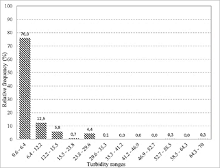
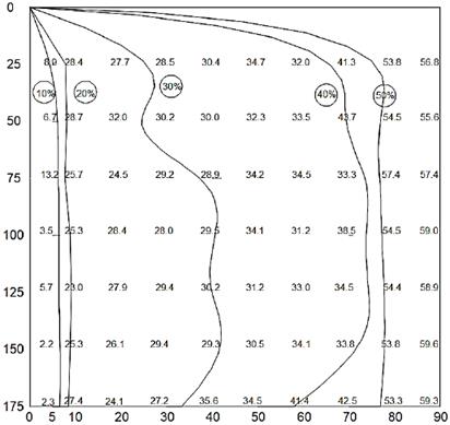
When the initial turbidity in the problem water is 2 NTUs (see Fig. 2), it is not possible to fit the curves to the dispersion of points obtained. The initial turbidity in the problem water is low and therefore, the flocculation coagulation process is affected due to the fact that the colloidal particles present in the water are dispersed and many of these do not become agglutinated by the coagulant. The dispersion coefficient in this case is the lowest, presenting a value of 0.63.

Source: The authors.
Figure 2 Isoconcentration curves for an initial turbidity of 2 NTUs. Vertical axis: Depth (cm). Horizontal axis: Time (min).
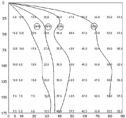
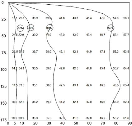
For the Figs. 3, 4, 5 and 6 the initial turbidity in the test water is 4, 6.1, 8.8 and 9.1 NTUs respectively. For these cases, the coefficient of determination R2 is less than 0.9 and therefore for these low initial turbidity values, the San's equation does not have a good fit to the field data.
Source: The authors.
Figure 3 Isoconcentration curves for an initial turbidity of 4 NTUs. Vertical axis: Depth (cm). Horizontal axis: Time (min).
Source: The authors.
Figure 4 Isoconcentration curves for an initial turbidity of 6.1 NTUs. Vertical axis: Depth (cm). Horizontal axis: Time (min).
Source: The authors.
Figure 5 Isoconcentration curves for an initial turbidity of 8.8 NTUs. Vertical axis: Depth (cm). Horizontal axis: Time (min)
Source: The authors.
Figure 6 Isoconcentration curves for an initial turbidity of 9.1 NTUs. Vertical axis: Depth (cm). Horizontal axis: Time (min).
The characteristic behavior of the Iso-concentration curves for type 2 settlers, when the initial turbidity in the problem water is high, shows that: i) for the same height, the longer the sedimentation time, the greater the removal efficiency, ii) for the same time, the deeper the sedimentation depth, the lower the removal efficiency. This trend can be observed in the studies referenced in Table 3.
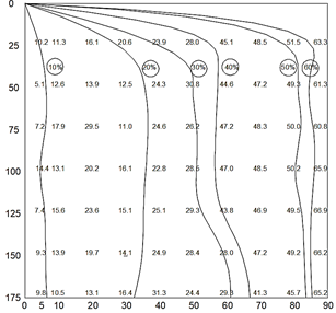
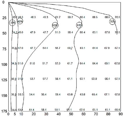
In the case of low initial turbidity values in the test water, as analyzed in the present study, the behavior of the Iso-concentration curves is affected by the low concentration of colloidal particles. In this case, for the same time, two depths of sedimentation can have the same particle removal efficiency. This can be observed in the behavior of the Iso-concentration curves shown between Figs. 3 - 6, where the curve that adjusts to the dispersion of points is no longer smooth and has an irregular behavior. For the Figs. 7 and 8 the coefficient of determination R2 is greater than 0.9 and therefore, the San's equation has a good fit to the field data.

Source: The authors.
Figure 7 Isoconcentration curves for an initial turbidity of 11.8 NTUs Vertical axis: Depth (cm). Horizontal axis: Time (min)
Source: The authors.
Figure 8 Isoconcentration curves for an initial turbidity of 14.9 NTUs. Vertical axis: Depth (cm). Horizontal axis: Time (min).
According to that reported by Aluminum & Salts [23] low turbidity waters are usually hard to coagulate due to low concentrations of stable particles and sometimes turbidity is synthetically added to the water to form heavier flocs which can be settled. The stability of the particles is related to the electrostatic forces, in this sense, for a colloid to flocculate, that is, to agglutinate with others, it is necessary for the particles to approach at a distance less than that between the center of the colloid and the crest of the resultant or energy barrier [18].
3.3 Analysis of the goodness of fit of the San equation as a function of the initial turbidity of the test water.
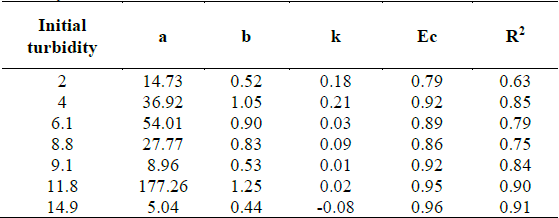
Table 4 shows the results of the San model constants, the values of the correlation coefficients (Ec) and the coefficient of determination (R2), obtained after performing the multiple linear regression with the data measured in the laboratory.
Table 4 Variation of the constants of the San model as a function of the initial turbidity.
Source: The authors.
In general, the correlation coefficient Ec is greater than 0.7 independent of the initial turbidity value in the test water. Ec values greater than 0.7 indicate that there is a high association between sedimentation depth and time (independent variables), with the percentage of removal of flocculent particles (dependent variable).
On the other hand, the coefficient of determination R2 indicates the degree of goodness of fit of the equations obtained through multiple linear regression, with respect to the data obtained in the laboratory. Considering that R2 values above 0.9 represent a good fit of the equation with respect to the sample values, it can be said that, for the case study, when the initial turbidity in the test water is less than 11.8 NTU, the San's equation does not have a good fit to the field data, making this a restriction for its application. Table 4 shows the values obtained for the different initial turbidity values.
Finally, the behavior of the constants a, b and k of the San model as a function of the initial turbidity is variable, showing that there is no clearly identifiable relationship between the initial turbidity and these constants. The foregoing would be associated with the behavior of water coagulation when turbidity is low, where said process is less efficient, given that, for low turbidity, the colloidal particles are more dispersed and it is more complex to agglutinate them with the use of the coagulant.
4. Conclusions
The frequency analysis of the historical turbidity data at the entrance of the four plants selected in the present study, allows to verify that a high percentage of the samples taken at the entrance of the treatment plants in operation, present low values of characteristic turbidity clear water and that can occur in the upper parts of the basins.
The mathematical equations that the different authors have developed to determine the percentage of removal of flocculent particles in a sedimentation tower, have been obtained with values of initial turbidity in the problem water between medium and high, evidencing that an analysis of the goodness of fit of these equations for low values of initial turbidity.
The analysis of the goodness of fit carried out with the San model for the present study allows us to verify that when the initial turbidity in the problem water is low (less than 11.8 NTU), the coefficient of determination R2 is less than 0.9 and therefore San's model does not show an adequate fit to the data measured in the laboratory. For lower turbidity values, the goodness of fit is lower.
There is a restriction in the use of the San model to determine the percentage of removal of flocculent particles and it is associated with low turbidity values in the test water. It is advisable to evaluate what happens with the goodness of fit of the other mathematical equations that have been developed, under the initial conditions in the problem water defined in the present study.

