


 Inglés (pdf)
 Articulo en XML
 Referencias del artículo
 Enviar articulo por email
 Citado por SciELO
  Citado por Google
  Similares en
SciELO
Similares en
SciELO  Similares en Google
 Permalink
1. Introduction
The classification of land-cover categories from remote sensing data is a task that has been developed for several decades [1-3]. Land-cover studies are relevant in different applications, including forest monitoring, water quality assessment, soil properties estimation, urbanization studies, among others [4-6].
The particular research on urban land-cover classification experienced a steady increase in the last decades since it is a relevant topic for communities, territorial entities, and local governments [7]. This increase was mainly due to the public availability of very-high-resolution imagery (VHR) since the late 1990s [8]. Although these VHR images are the primary input data for this type of study, because of the heterogeneity of the urban environment, medium and low-resolution images do not allow to discriminate small and common elements such as trees, buildings, cars, and even people [2]. Furthermore, using these VHR images also poses technical challenges due to the internal spectral and spatial heterogeneity within urban land cover categories [9].
Urban land-cover classification from remote sensing images is traditionally based on differences between pixel-level spectral responses [1]. However, this approach has problems when the size of the objects under study is larger than the spatial resolution of the image [10]. Additionally, due to the high spectral variability of urban land-cover in VHR images, such an approach for classification generally obtains low accuracies due to effects such as salt and pepper or structural clutter [7]. It also highlights the most crucial problem of this type of classification, which ignores intrinsic urban land cover characteristics, such as spatial environment, geometry, and context [11].
The limitations mentioned above create the need to restructure how VHR image classification has been approached. The change from the basic unit of study, the pixel, to another unit, the object, can account for both spatial and spectral characteristics. Currently, apart from the per-pixel approach, the most widely used approaches for land-cover classification are the per-field, object-based, contextual-based, knowledge-based, and combinational approaches [12].
Blaschke and Strobl [13] state that the change from pixel to object, as a basic unit in remote sensing image analysis, significantly improves classification results, even in complex scenarios represented in VHR images. These objects are analyzed using concepts and techniques recently developed, which contribute to defining the Geographic-Object Based Image Analysis (GEOBIA) for land cover classification [8,12,14].
These techniques segment images and generate image objects created from groups of neighboring pixels, which are similar to each other or share some common meaning [15]. In addition to the spectral response of the objects, it also considers their spatial, textural, temporal, multi-scale, geometric, and contextual characteristics, a crucial aspect for the classification of urban land-cover [16,17]. These objects are created within the GEOBIA workflow by three main stages: segmentation, which groups pixels to form objects; feature analysis which extracts relevant attributes from objects; and classification, which evaluates and decides the land-cover class to which the object belongs [18,19].
Research like that of Myint et al. [10] compared the performance of pixel- and object-based methods in an urban environment using VHR images, finding that the overall accuracy of object-oriented classification improves by around 27% compared to pixel-based classification. This is primarily due to the advances these methods have had in enhancing their segmentation and classification phases.
Segmentation is the crucial process of GEOBIA methods [9]. A great variety of algorithms carry out this activity, including Mean Shift, Chessboard, Quadtree, Contrast Split, Spectral Difference, or Contrast Filter [20]. However, the vast majority of investigations related to the classification of VHR images in urban environments agree that the multi-resolution segmentation (MRS) algorithm is the one that obtains the best results [21]. The principle of this algorithm is the grouping of pixels through seeds distributed throughout an image based on criteria established by its hyperparameters scale (SP), Shape, and Compactness [22]. Its great advantage is that it produces objects with high internal homogeneity more efficiently than other segmentation methods [21], essential for the final land-cover classification.
On the other hand, the classification algorithms performing best within GEOBIA are Machine Learning (ML) algorithms. Among these, the one that has obtained the best results is Random Forest (RF) [23]. RF is a structured collection of decision trees, where each tree is built with data and variables chosen at random. Then, each casts a vote regarding a given classification, and the result with the highest number of votes is the final prediction [24]. Its most favorable characteristic is that it only needs to configure a few parameters for its operation. As a result, it is faster than other ML algorithms, such as support vector machines or artificial neural networks [25].
Ruiz Hernández and Shi [26] conducted GEOBIA classification using the MRS and RF algorithms to map urban land-cover with VHR images, obtaining overall thematic accuracy results of 92.3%. Similarly, Baker et al. [27] classified urban domestic gardens, combining VHR image data with vector data, obtaining an overall thematic accuracy (OA) of 82%. However, these two studies did not conduct any tuning of the GEOBIA phases, which could have caused the results obtained not to reach higher accuracy.
The scope of this paper is to compare the overall accuracy obtained by two workflows based on GEOBIA, one non-optimized and the other with optimizations in each phase. The International Society for Photogrammetry and Remote Sensing (ISPRS) provides the input data used and the ground truth to evaluate the results [28].
The central hypothesis is that optimizing the phases of a workflow based on GEOBIA improves the overall accuracy and the efficiency of the process. The main contributions of this paper are: (i) it demonstrates that the inclusion of relevant variables and object attributes derived from primary data improves the overall accuracy of urban land-cover classification; (ii) it establishes the impact the optimization of the segmentation and classification phases has on the overall accuracy of the workflow; and (iii) it demonstrates the importance of implementing a general optimization of the phases of a GEOBIA workflow, as a good practice in the urban land-cover classification. Optimization of the image classification process means paying attention to all phases of the GEOBIA approach, that is, (i) image segmentation, (ii) feature selection, and (iii) image classification.
This article is organized as follows. Section 2 presents and describes the study area, the input data, and the methods used to extract urban land-cover categories. Section 3 presents the results obtained using the described methods. Section 4 discusses the results found, and Section 5 presents the conclusions obtained from the research.
2. Data and methods
2.1 Study area
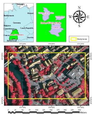
The study area is located in Vaihingen an der Enz, a small town in the Ludwigsburg district of the federal state of Baden- Wurttemberg in Germany (Fig. 1). It is northwest of the city of Stuttgart; an urban area characterized by residential and recreational land use [28]. Although its urban structure presents low-rise buildings that are widely separated from each other, it also shows a large amount of urban vegetation (rows of trees, bushes, and grass). This structure represents a typical old town in Germany [29].
2.2 Data
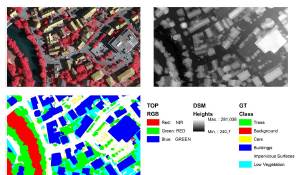
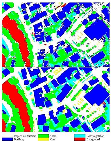
The study area is subdivided into 33 areas distributed in the city center, from which true orthophotos (TOP), digital surface models (DSM), and ground truth (GT) of the surface objects corresponding to area 26 were taken (Fig. 2). The dataset is a subset of the data used for the digital aerial camera test performed by the German Association of Photogrammetry and Remote Sensing (DGPF) [30].
Source: The authors.
Figure 2 Data set from Area 26. Top-Left: True Orthophoto. Top-Right: Digital Surface Model. Bottom-Left: Ground Truth
2.1.1 True Orthophoto (TOP) and Digital Surface Model (DSM)
The process of acquiring the images necessary to generate the TOPs and DSMs was carried out and coordinated by the Institute of Photogrammetry of the University of Stuttgart under the supervision of the DGPf. It was carried out by executing a flight plan of seven strips, with a block with five parallel and overlapping strips and two crossed strips at the ends of the block [29]. The flight days for taking the images were July 24 and August 6, 2008, and a DMC camera from the Intergraph/ZI company was used [30]. Once the DGPF took the aerial photographs, Rottensteiner et al. [29] generated a TOP and DSM of the entire study area, from which individual TOP and DSM were extracted for each of the 33 areas. The TOP and DSM specifications for area 26 are described in Table 1.
2.1.2 Ground Truth (GT)
The GT was obtained from ISPRS [28] in TIFF files with three bands (red, green, and blue - RGB), which were only assigned values of 0 and 255, this to be able to encode the six classes in which the areas are classified and described in Table 2.
Table 2 Land-cover classes description.
| Class Number | Class | RGB coding | Colour |
|---|---|---|---|
| 1 | Impervious Surfaces | 255, 255, 255 | White |
| 2 | Buildings | 0, 0, 255 | Blue |
| 3 | Low Vegetation | 0, 255, 255 | Cyan |
| 4 | Trees | 0, 255, 0 | Green |
| 5 | Cars | 255, 255, 0 | Yellow |
| 6 | Background | 255, 0, 0 | Red |
Source: The authors.
The urban land cover classes used here are the most commonly found in an urban environment. The impervious surface class included roads, pedestrian paths, parking lots, and all kinds of surfaces made of asphalt or concrete at ground level. The building class covered the entire estate spectrum, such as houses, warehouses, and any residential, commercial, industrial, or institutional structure found. The Low vegetation class refers to all biomass found at ground level, for example, grass, living fences, or small shrubs. The tree class covered all the large vegetation existing in the areas. The car class contained all the fleet of vehicles that could be found. Finally, the background class included water surfaces and other objects that look different from everything previously classified (swimming pools, containers, tennis courts, among others) [28].
The training and validation processes samples were taken through a stratified random sample, where each stratum is equivalent to each of the urban land-cover classes. Simple random sampling was carried out for each stratum. 30% of the total area 26 was taken for the training process, and the remaining 70% was used in the validation.
2.3 Method
The GEOBIA-based workflow shown in Fig. 3 was divided into two parts. A non-optimized workflow takes default values in each phase of the workflow and another with the proposed optimization. In each phase, variables, attributes, and hyperparameters are added or optimized as the case may be. Both workflows comprise four main phases and a preprocessing phase: In phase 0, the variables derived from TOP and DSM were calculated; in phase 1, the segmentation process was carried out using the MRS algorithm; in phase 2, the object's features were calculated; in phase 3, the RF algorithm was used to carry out the classification; In phase 4, the classification obtained was evaluated by calculating the confusion matrix and its accuracy indexes.
2.3.1 Phase 0: Preprocessing
First, the position, scale, and orientation verification of the TOP and DSM of area 26 were carried out.
For the optimized GEOBIA workflow, variables derived from TOP and DSM were calculated, such as textural variables from the gray level co-occurrence matrix (GLCM) [31]; the normalized digital surface model (nDSM); the slope [32], and the normalized difference vegetation index (NDVI) [33].
The GLCM textural variables calculated were Contrast (CON), Dissimilarity (DIS), Homogeneity (HOM), Angular Second Moment (ASM), Entropy (ENT), Mean (MEN), Standard Deviation (STD), and Correlation (COR). These variables are defined as shown in eq. (1)-(8) respectively
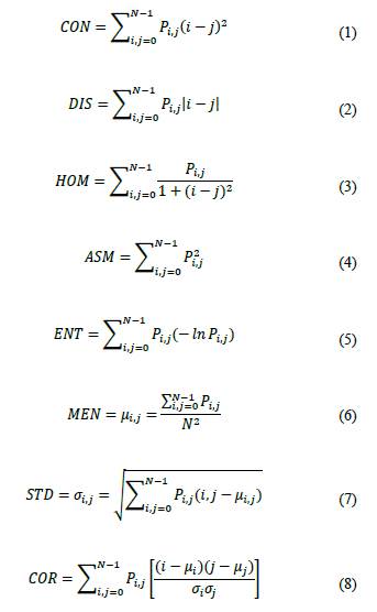
where i, j represent the number of rows and columns of GLCM, P i,j is the probability in the pixel i, j, and N is the number of rows or columns of GLCM. Variables such as CON, DIS, ENT, and STD show the local variation degree in an image. For their part, variables such as HOM, MEN, COR, and ASM are a measure of image homogeneity [31].
The nDSM represents the relative height to the ground of objects above the earth's surface and is defined as shown by eq. (9).
where DSM, is the digital surface model and DTM, is the digital terrain model.
Slope is the inclination of a given point on a topographic surface [32]. This was calculated from the DSM according to eq. (10),
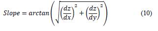
Where
 describes the elevation change Z in the direction, respectively.
The NDVI is the vegetation index most used in urban land-cover studies since it allows differentiation of vegetal land-cover from other present land-cover classes [7]. Its calculation is established by the difference of reflectance in the infrared and red bands divided by their sum, as shown in eq. (11).
where NIR and RED are reflectance values in the TOP image corresponding to near-infrared and red bands, respectively.
2.3.2 Phase 1 - Segmentation
In this phase, the MRS algorithm implemented in the eCognition 9.0 software was used [34]. For the non-optimized workflow, the default values of the SP, Shape and Compactness hyperparameters were used (10, 0.1 and 0.5, respectively). This phase's optimization consisted of determining the best value combination of the three hyperparameters through several iterations. The typical land-cover sizes in the scene were considered in the Sp setting, especially the car land-cover, the smallest of all. The Shape and Compactness hyperparameters vary between 0 and 1; however, in this phase, values between 0.1 and 0.9 were taken for both according to recommendations from previous studies [34]. To observe the behavior of Shape and Compactness, high, medium, and low values were taken.
2.3.3 Phase 2 - Feature Analysis
The features or attributes calculated for each object output by the segmentation phase correspond to the textural type (GLCM); geomorphometric (DSM, nDSM, and Slope), and spectral (TOP, NDVI, Max.Diff, and Brightness), as shown in Table 3. Max.Diff and Brightness were calculated according to the terms of [34].
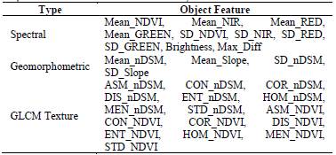
First, for the non-optimized workflow, Mean NIR, Mean RED, Mean GREEN, and Mean DSM attributes were calculated in each object generated by the segmentation.
Feature analysis for workflow optimization comprises calculating spectral, geomorphometric, and textural features for each object. Feature selection was then carried out using the Regularized Random Forest (RRF) [35-37] and Recursive Feature Elimination (RFE) algorithms [38]. These algorithms make it possible to select the best group of features, considering elimination parameters such as redundancy or collinearity between them [39]. In addition, this phase sought to find the attributes set that produced the best accuracy in the final classification, minimizing the problems associated previously. For the GRRF and GRF algorithms, the gamma penalty parameter ranged from 0.1 to 1 [36,37].
2.3.4 Phase 3 - Classification
Before entering the classification phase, the training and test samples selection was carried out as stated in section 2.2.2.
The RF algorithm was implemented for the classification phase. To evaluate the data and variables' performance, RF uses two importance indexes, Mean Decrease Accuracy (MDA) and Mean Decrease Gini (MDG). MDA measures the overall accuracy reduction of RF concerning the absence of a given variable, and MDG accounts for the impact that excluding a variable has on the rapid choice of the decision tree [25].
RF was initially run without optimization, using the default values for its hyperparameters: number of trees (ntree), number of attributes for each tree (mtry), and minimum node size to be divided (min.node.size), within the R randomForest library [40]. Subsequently, the RF hyperparameters were adjusted simultaneously by successive iterations between possible value combinations. Following Belgiu and Dragut [25], the values of the RF hyperparameters were chosen as follows: ntree values less than 500, mtry values greater than 5, and min.node.size values greater than 1.
2.3.5 Phase 4 - Validation
For the validation, the confusion matrix was calculated, a square matrix whose numerical values in the rows and columns represent the number of study units assigned to a given class, based on the GT reference classification [41]. The overall accuracy index (OA) and F1-score index are calculated to quantify the obtained accuracies from the confusion matrix, as shown in eq. (12,13) respectively
where TP are the correctly classified objects; TN, the correctly non-classified objects; FP, the classified objects in a class that was not the true one; and FN, the non-classified objects in the true class [42].
3. Results
3.1 Non-optimized workflow implementation
Table 4 shows the input data values for each phase described above, taken without making adjustments or processing.
Table 4 Default values for non-optimized workflow input data.
| Input Data | Default Value |
|---|---|
| Variables | NIR, RED, GREEN, DSM |
| MRS Hyperparameters | SP=10, Shape=0.1, Compactness=0.5 |
| Feature Objects | Mean_NIR, Mean_RED, Mean_GREEN, Mean_DSM |
| RF Hyperparameters | ntree=500, mtry=5, min.node.size=1 |
Source: The authors.
In phase 0, we do not perform processing on the TOP and DSM bands, which we take as input data for segmentation. For phase 1, we use the default values of MRS algorithm to generate the segmented objects. In phase 2, we calculate the object attributes corresponding to the mean response of each variable in each object.
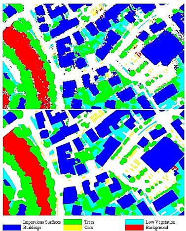
For phase 3, we trained RF with 30% of the objects obtained, and we used the default values of the R randomForest library. Then, we carried out the classification with the remaining 70% of the objects, and we obtained the result shown in Fig. 4.
Source: The authors.
Figure 4 Non-optimized workflow classification results for Area 26. OA = 77.68%. Top: Final classification. Bottom: GT.
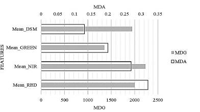
The MDA and MDG importance indexes are shown in Fig. 5, where it is revealed that the best attributes are MeanNIR and MeanRED. MDA values of 0.32 and 0.27 for MeanRED and MeanNIR, respectively, indicated the decreased degree in accuracy with the absence of these attributes. On the other hand, MDG values of 2230 and 2000 for MeanNIR and MeanRED, respectively, indicated the impact that the exclusion of the attribute has on the speed of the RF decision in the classification.
The overall accuracy for the non-optimized classification workflow is shown in Table 5, where after evaluating the confusion matrix, we calculated the OA and the F1-score indexes for each land-cover class.
Table 5 Summary of classification accuracy indexes.
| Class | F1-score (%) |
|---|---|
| Impervious Surfaces | 73.89 |
| Buildings | 83.49 |
| Low Vegetation | 49.51 |
| Trees | 88.14 |
| Cars | 31.75 |
| Background | 68.84 |
| OA (%) | 77.68 |
Source: The authors.
We observe that the OA of the classification is 77.68%, where the classes with the highest thematic accuracy (F1-score) are Trees, Buildings, and Impervious Surfaces with 88.14%, 83.49%, and 73.89% values, respectively. On the other hand, we found that the lowest F1-score values were presented in the Cars, Low Vegetation, and Background classes with 31.75%, 49.51%, and 68.84% values, respectively.
3.1.1 Optimized workflow implementation
The workflow optimization is carried out for each phase, and in each one, we evaluate the OA applying the workflow of section 3.1 with the accumulated optimizations per phase.
3.1.2 Phase 0 - Preprocessing
We calculate three types of derived variables from the input variables: spectral, geomorphometric, and texture, which are listed in Table 6.
Table 6 Summary of input data variables.
| Type | Variable |
|---|---|
| Spectral | NDVI, NIR, RED, GREEN |
| Geomorphometric | nDSM, Slope |
| GLCM Texture | MEN, STD, HOM, CON, DIS, ENT, ASM, COR |
Source: The authors.
For the GLCM texture variables calculation, we chose a 3X3 window size and the NIR variable. Then, we calculate the OA of the inclusion of the new variable, evaluating first the inclusion only of GLCM textural variables, then only the geomorphometric and spectral variables, finally, the entire set of variables with a result 81.78%, 82.39 %, and 84.59% respectively.
3.1.3 Phase 1 - Segmentation
Table 7 shows the different values used for the MRS hyperparameters adjustment. We evaluate each combination of values using the non-optimized workflow developed in section 3.1, including the NDVI, NIR, RED, GREEN, nDSM, Slope, MEN, STD, HOM, and CON DIS, ENT, ASM, and COR variables calculated in section 3.2.1.
Table 7 MRS hyperparameters values.
| MRS Hyperparameter | Values |
|---|---|
| SP | 10, 12, 14, 16, 18, 20 |
| Shape | 0.1, 0.5, 0.9 |
| Compactness | 0.1, 0.5, 0.9 |
Source: The authors.
We obtained 54 possible combinations of hyperparameters. The best result was obtained with the values of SP = 10, Shape = 0.9, and Compactness = 0.9 with an OA = 86.63%.
3.1.4 Phase 2 - Feature Analysis
We calculate a total of 30 object attributes from the entered variables and evaluate their performance by applying the optimizations of phases 0 and 1 to the workflow of section 3.1. Table 8 shows the results and the number of attributes selected for each algorithm used.
Table 8 Feature selection results. GRRF and GRF, the gamma penalty parameter was varied from 0.1 to 1 according to [36, 37]. Time is the processing time of each algorithm.
| Algorithm | # Features | Time (s) | OA (%) |
|---|---|---|---|
| RF | 30 | 127.81 | 86.67 |
| RRF | 30 | 227.45 | 86.77 |
| GRRF (0.1) | 30 | 1680.24 | 86.80 |
| GRF (0.1) | 30 | 1170.76 | 86.78 |
| RFE | 17 | 98159.01 | 86.84 |
Source: The authors.
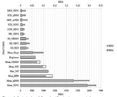
We found that the best result was obtained with the RFE algorithm with an OA = 86.84% and a feature set size of 17. Next, we evaluate the performance of the selected attributes as shown in Fig. 6, where the attributes with the highest incidence in the classification were Mean NDVI and MeannDSM.
3.1.5 Phase 3 - Classification
Once the optimal set of attributes was obtained, we adjusted the RF hyperparameters for subsequent classification. We simultaneously adjusted the ntree, mtry and min.node.size hyperparameters , whose values can be seen in Table 9.
Table 9 RF hyperparameters values.
| RF Hyperparameter | Values |
|---|---|
| ntree | 200, 250, 300, 350, 400, 450, 500 |
| mtry | 6, 7, 8, 9 |
| min.node.size | 2, 3, 4, 5, 6, 7, 8, 9 |
Source: The authors.
We evaluated 224 combinations of hyperparameters entirely, from which we obtained two combinations with the best performance, as shown in Table 10.
Table 10 RF hyperparameters combinations with the best result. Time is the
| Combination | ntree | mtry | min.node.size | OA (%) | Time (s) |
|---|---|---|---|---|---|
| C1 | 350 | 9 | 4 | 87.02 | 104.00 |
| C2 | 450 | 9 | 3 | 87.02 | 133.86 |
Source: The authors.
We chose the C1 combination because it has the shortest processing time. Therefore, we obtained the final classification with this combination, and the result is shown in Fig. 7.
3.1.6 Phase 4 - Validation
We evaluate thematic accuracy indexes for the classification and compare the results with those of the workflow in section 3.1. Table 11 shows the overall accuracy value and F1-score values for each land-cover class.
Table 11 Summary of classification accuracy indexes.
| Class | F1-score (%) |
|---|---|
| Impervious Surfaces | 83.80 |
| Buildings | 92.92 |
| Low Vegetation | 71.64 |
| Trees | 91.56 |
| Cars | 52.89 |
| Background | 83.83 |
| OA (%) | 87.02 |
Source: The authors.
We obtained an OA value for the classification of 87.02%. The land-cover classes with the highest thematic accuracy (F1-score) ate Buildings, Trees, Background and Impervious Surfaces with92.92%, 91.56%, 83.83%o 83.80%, respectively. Moreover, we found that the lowest values of the F1-score were presented in the Cars and Low Vegetation classes, with values 52.89% and 71.64%, respectively.
4. Discussion
We compared the overall accuracy values between the non-optimized and optimized workflow and found an increase in OA of 9.34%. In addition, we showed that the optimization of each phase of a GEOBIA workflow significantly increased the accuracy of the land-cover classification in VHR images.
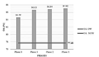
Fig. 8 shows the variation of the OA increase of the workflow as each phase was optimized. Starting from the OA reference of the non-optimized workflow (77.68%), successive increases in OA were observed as each phase was optimized, with values 6.91%, 2.04%, 0.21%, and 0.18% for phases 0, 1, 2, and 3, respectively.
Source: The authors.
Figure 8 OA increases in each phase (OA OW = OA Optimized Workflow, OA NOW = OA Non-Optimized Workflow).
The optimized phase that most contributed to the increase in OA was phase 0, where it was evidenced that, by themselves, variables such as GLCM texture or NDVI and nDSM increased OA by 4.1% and 4.71%, respectively. The above demonstrated the importance of the preprocessing phase and the appropriate choice of variables derived from the input data, confirming the conclusions reached by Salehi et al. [7] and Jennifer et al. [43].
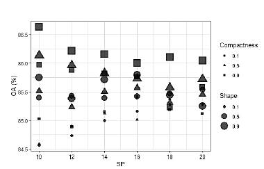
The optimization process of the MRS hyperparameters showed the importance of choosing their best possible combination. For example, fig. 9 shows the distribution of OA through the 54 combinations of hyperparameters, where it was found that the combinations with higher and lower OA were obtained with SP = 10, indicating that the mere fact of adjusting SP does not ensure the best possible segmentation [6,44].
From 30 calculated object features, a set of 17 features was selected as the most optimal, considering that RFE chose this number of features based on the best accuracy result among all possible features subsets, and in this subset, the importance indexes of each feature were calculated. Fig. 6 shows that the most relevant object feature was MeanNDVI and MeannDSM. These attributes presented differences in importance index values regarding the other attributes of 0.15 (MDA) and 4160 (MDG) for Mean NDVI and of 0.09 (MDA) and 3560 (MDG) for MeannDSM. Otherwise, the object features with the lowest performance were those of GLCM texture. Only 6 of the 14 calculated ones were selected for the final classification, and these six presented the lowest performance. These results support the findings from the study by Aguilar et al. [45] and Aguilar et al. [46], whose objective was to demonstrate the VHR images potential to classify urban land-covers through different classes of variables, and where it was established that the spectral indexes and the relative heights to the ground (OA=83.6%), help to better classify the urban land-covers, in comparison with the texture measurements (OA=77.9%).
Regarding the feature selection algorithms, the most significant difference between the OAs reported in Table 8 was 0.17%, between the RFE algorithm and RRF family algorithms, in contrast to the processing times, where RFE had an increase of 59 times (approximately 27 hours) compared to the RRF family algorithms. These results showed that although the RFE algorithm presented the best performance, its computational cost is not comparable with that of the RRF algorithms' family. Processing time was calculated using a computer with a four-core processor, each with a 2.20Ghz processing speed and 8GB RAM.
The RF hyperparameters optimization found that in the 224 combinations performed; the OA had a maximum variation of 0.19%. Therefore, it was demonstrated that RF is a robust ML method that is not affected by its performance by the hyperparameters adjusting [25,47]. However, we found that this setting improved the workflow processing time, especially the ntree setting. Fig. 10 shows that the processing time can be up to four times longer, depending mainly on the value of ntree. This result confirms the finding of Probst et al. [48], where after a certain ntree value, the OA stabilizes so that an increase of this kind only increases the processing time. Conversely, for mtry and min.node.size, no indication was found in the results confirming the increase in OA suggested by Probst et al. [48].
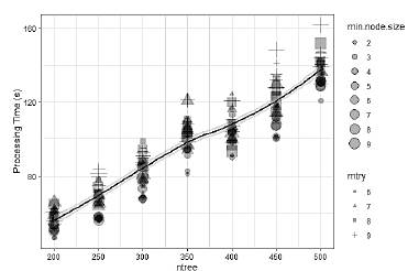
Source: The authors.
Figure 10 Time processing distribution for the RF hyperparameters combinations.
Finally, we observed F1-score index value increases of 9.91%, 9.43%, 22.13%, 3.42%, 21.14, and 14.99% in the land-cover classes, Impervious Surfaces, Buildings, Low Vegetation, Trees, Cars and Background, respectively. These results showed that the overall workflow optimization had a greater impact on classes such as Low Vegetation, Cars, and Background. However, the OA values are lower with respect to the other classes, so it is found that there are land-cover classes that are more sensitive to the GEOBIA optimization
5. Conclusions
The results obtained in this research confirmed that spectral, geomorphometric, and texture variables derived from primary data improve the quality of the VHR image segmentation process in urban environments. Furthermore, as demonstrated, including these variables in the process before segmentation increased the GEOBIA workflow overall accuracy by 6.91%. This figure was the largest increase per phase, so special attention must be paid to the type of input data and possible variables derived from these, according to the kind of land cover to be classified.
The MRS hyperparameter optimization in the segmentation phase allowed establishing the importance of this adjustment in the resulting objects. The literature consulted gives more importance to the SP hyperparameter, however, it was found that the appropriate choice of Shape and Compactness values can increase the OA of the workflow by up to 2%.
The RF hyperparameters optimization and feature selection in the classification phase indicated an incidence in the processing times more than in the OA of the workflow. The ntree hyperparameter was found to be the most relevant, so it is advisable to set it around 350 to improve processing time.
Finally, research results demonstrated the importance of implementing optimization processes in GEOBIA workflows, the increase of around 10% in OA verified that this activity should not only be adopted as good practice but should be thoroughly analyzed depending on the case study.

