English (pdf)
 Article in xml format
 Article references
 Send this article by e-mail
 Cited by SciELO
  Cited by Google
  Similars in
SciELO
Similars in
SciELO  Similars in Google
 Permalink
1. Introduction
Hydrocarbon reserves in unconsolidated or weakly consolidated formations represent 70% of world reservoir reserves [1]. During the production of these reservoirs, sanding frequently occurs, which increases the operational risks in wells and on surface facilities as well as the costs for remediation and cleaning operations. To prevent and control sanding, mechanical filters are used, which are costly and reduce productivity [2].
Sanding occurs when the drag forces exerted on a matrix by flowing fluids (during production) are greater than the resistive forces of the formation grains. Different factors influence these forces, such as rock and fluid properties, stress state around the well, and type of completion used [2]. In a model, the inclusion of all mechanisms and factors that influence sanding can result in a very complex numerical model. Thus, developing a model with lesser constraints and assumptions is necessary to analyze the most relevant mechanisms and to forecast the sand-production potential of formations in order to design a process for optimum completion of a well, optimize production, and avoid setbacks in future operations [2]. Therefore, to study sanding and its mechanisms, we need to use models that reproduce the actual behavior of the fluids and rocks [3].
The present study develops a mathematical and computational model. This model attempts to estimate the onset of sand production and quantify the rate of sand production for nonconsolidated or weakly consolidated formations. This study recognizes the importance of using an elastoplastic constitutive model to simulate the mechanical behavior of rocks. In addition, it demonstrates how the proposed model helps to perform better analysis of the sand-production phenomenon under laboratory conditions. This process is important for adjusting the parameters associated with elastoplastic behavior, including adjustment of the parameters related to porosity and permeability evolution.
Despite the current developments in sand-production modeling, the relationship between sand production and porosity-permeability of a material remains unclear. Furthermore, the mechanical behavior of sanding occurrence is not fully understood. Consequently, this study introduces a numerical model that includes current developments related to the effect of sand production on porous volume, porosity, permeability, and fluid-rate calculations.
2. Literature review
During oil and gas production, the reservoir formations are subjected to high seepage forces and sand is produced, along with the produced fluids. The literature provides two main types of models for modeling the sand-production phenomena, namely, models based on the continuum and discontinuum approaches. In addition, the solutions based on continuous mechanics consist of analytical and numerical solutions [2]. The current study focuses on the numerical models based on the continuum approach.
The numerical models use the following equations for the solutions: solid-mass balance, fluid-mass balance, and force equilibrium. These models result in a system of equations that represents the sanding phenomenology.
Early models for sanding quantification highlighted the importance of the erosional phenomena. One of the very first models stated that the volumetric solid production is a function of the erosional rate, and this erosional rate depends on the fluid velocity and solid concentration in the flow phase (eq. 1) [4].
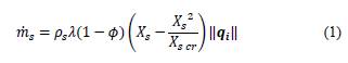
where ṁ s is the sand-mass rate, p s is the solid density, 𝜙 is the porosity, X s is the concentration of solids in the moving fluid, X s cr is the critical solid concentration, and q i is the fluid-discharge rate.
An additional model defines the minimum fluid-velocity expression for the onset of solid production, which is defined as a function of the residual resistance and petrophysical properties [5]. The additional model includes elastoplasticity as a fundamental behavior of sanding mean, whereas the solid concentration is eliminated in eq. (1). The elastoplastic phenomena are included in the λ variable, which assumes two components: a minimum plasticization level to trigger solid production and the evolution of parameter λ proportional to the plastic strain until it reaches a maximum value [6]. Different researchers employ the minimum plasticization level for the sanding onset using experimental or numerical methods [7-9].
Several studies include sand production in their calculations and confirm that the sand-production level is related to the plasticized volume of a formation [10]. Additionally, three conditions that trigger the production of sand are proposed [11]. First, sanding occurs only at the cavity faces. Second, the element must have zero cohesion and be under tension condition. Third, the model removes the sanded element from the grid. Another assumption for the sanding models is that an element is eroded when it does not satisfy the equilibrium equations [12,13].
Another sand-production criterion is the requirement for a critical level of plastic deformation and fluid velocity to transport the detached grains [14]. The effect of the three-phase flow and capillary forces in the critical fluid velocity on sand production has also been investigated [15]. Another model introduces a pressure-gradient criterion at the pore scale for onset prediction [16]. However, this criterion is derived by mechanical analysis at the pore scale; thus, the geomechanical effect of stresses around the wellbore is not considered. In general, although, all previous models are based on force-equilibrium equations, fluid-mass balance, and solid-mass balance, they differ in the method in which sand is produced, effects of the produced sand, and involved constitutive equations.
The model presented in this research allows to asset the sand production onset and quantify the produced sand due to mechanical effects, as well as to study the effect of sand production on porosity-permeability relationship and its impact of hydrocarbons production rate, which leads to a general view of the causes and consequences of sand production.
3. Model specifications
3.1 Physical model
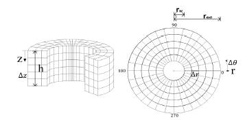
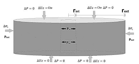
According to the problem's geometry, the simulation-domain geometry is a hollow cylinder with internal radius rw, external radius r ext , and thickness h (Fig. 1). This physical model is discretized in the r, 𝜃, and z directions depending on the number of required elements. In this domain, fluid flow and rock deformation simultaneously occur. The modeled formation is characterized as having high porosity, permeability, and deformability. This physical model incorporates boundary conditions similar to real conditions, such as stress at the inner radius, absence of flow at the top and bottom boundaries, and constant regional stresses at the borders of the reservoir.
3.2 Differential and numerical models
The differential model consists of fluid-flow, coupled geomechanical deformation, and sand-production models.
3.2.1 Fluid-flow model
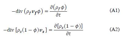
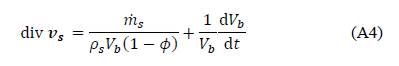
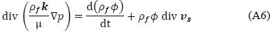
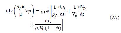
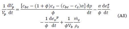
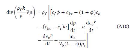
The fluid-flow model consists of the integration of the fluid- and solid-mass conservation equations with the monophasic diffusivity equation (Darcy's law) for a slightly compressible fluid. These equations, including the effects of porosity changes due to strain and solid production, result in the final equation for the fluid-flow model (eq. 2). The derivation of the fluid-flow model is shown in Annex A.
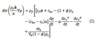
where p f is the fluid density, k is the permeability tensor, 𝜇 is the viscosity, p is the pressure, 𝜙 is the porosity, c f is the fluid compressibility, c bc is the bulk compressibility, c s is the solid compressibility, α is the Biot constant, t is the time, e v e is the elastic volumetric strain, e v p is the plastic volumetric strain, ṁ s is the mass rate of sand production, V b is the bulk volume, and p s is the solid density.
3.2.2 Geomechanical-deformation model
During the injection and production processes at the wellbore or the loading and unloading processes in the laboratory tests, the reservoir deforms. To develop a coupled model, three components must be integrated, namely, the stress-equilibrium equation (eq. 3), strain and displacement compatibility conditions (eq. 4), and constitutive model that integrates the stresses, strains, and pressure (eq. 5) [17].
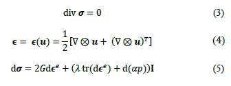
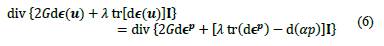
where 𝝈 is the total stress tensor, Є is the total strain tensor, u is the displacement vector,G is the shear modulus, λ is the Lame coefficient, and I is the Kronecker delta. The geomechanical-deformation model for a porous medium with elastoplastic behavior (eq. 6) is obtained from the introduction of eq. (4)-(5) into eq. (3), which yields a model that considers the pressure and plastic strains.
The plastic strains (dЄp) are calculated during material yielding. Then, the displacements are recalculated so that the new calculated stresses satisfy the condition f s (σ i ' N ) = 0. Among the different failure criteria, the Mohr-Coulomb criterion is the most conservative in its predictions, for this reason, Mohr-Coulomb criterion used in this model (eq. 7).
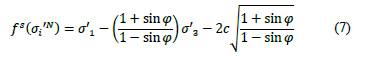
where σ’1 and σ' 3 are the maximum and minimum principal effective stresses, respectively, φ is the internal friction angle, and c is the cohesion of the material.
3.2.3 Hardening and softening parameters
The presented model uses the shear-hardening parameter (e ps ) for the accumulation of the shear plastic strains to quantify the level of mechanical damage due to shearing.
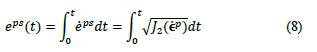
where ė ps is the rate of e ps , J 2 is a tensor invariant, and Ė p is the rate of the plastic-strain tensor.
3.2.4 Sand-production model
This section defines the sanding onset conditions and the amount of produced sand. Sand onset occurs at a specific level of plastic strain, which is known as the critical level of plastic failure (ecr ps). ecr ps = 0 implies that sanding onset occurs immediately after "plasticity" starts, which is a common assumption of the analytical models.
This model assumes that sand is produced only from the cavity faces exposed to fluid flow because sand production is an erosive phenomenon and the eroded grains are large; thus, sand cannot come from inside the reservoir. An innovative element in this model is the relationship between the mass of produced sand and level of plastic failure e ps . This relationship suggests that the amount of sand available for production is proportional to the level of plastic failure associated developed in the porous medium. Finally, the model establishes a minimum flow velocity for the detached grains to be transported by the fluid, i.e., sand is only produced when the fluid velocity exceeds the critical value to transport it ( v f > v f min ). Considering the abovementioned conditions, the rate of sand production is defined as:
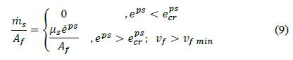
Where μ s is an experimental parameter. A f is the area of the sand-producing zone perpendicular to the flow and helps define a specific sand-production value (sand production per unit area), which can be used to extrapolate the results to cases such as wellbores and perforation tunnels.
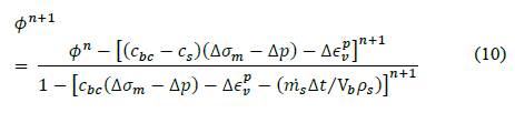
In eq. (9) a high flow velocity does not imply that solids are being produced. In other words, a solid matrix must be subjected to a certain plastic state and a flow velocity for the solids to be produced. Under sand-production conditions, an increase in the level of plasticity (e ps ) represents an increase in sand production. In eq. (10), the new porosity (𝜙 n+1 ) is a function of the mean stress, pressure, strains, and sand-production changes.
3.3 Initial and boundary conditions
As initial conditions, the pressure at each calculation node is equal to the initial pressure, besides, the initial displacements and plastic strains are equal to zero (eq. 11) (condition of an intact reservoir). The initial-stress state distribution includes axial and horizontal stresses with an isotropic stress condition at the horizontal plane (eq. 12).
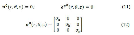
where u° is the initial displacement vector. In terms of the boundary conditions, the fluid-flow model denotes the pressure at the inner (p W f) and outer (p e ). Meanwhile, the solution uses no-flow boundary for the top and bottom boundaries. The boundary condition for the geomechanical model at the inner radius is σ rr = p wf , whereas that at the outer radius is Δσ rr = 0. Meanwhile, the top-boundary vertical displacement is set equal to zero.
3.4 Computational model
The proposed model is built in-house using the FORTRAN programming language. In addition, it is solved using the finite difference, fully coupled, and iterative method. The solution of the coupled system includes two convergence levels. In the first level, the solution of the pressure and displacement is obtained. When the first convergence level is finished, the stresses at time t n+1 are calculated, and the plasticity module evaluates the plastic deformations. In this manner, the second convergence level considers the plastic strains in the solution (see Fig. 2).
4. Sand-production-phenomenon modeling
The fundamental step is the matching of the results of the proposed model with real data, which can be achieved using either the laboratory or field data. In this study, the results of an experimental sand-production test are used [18]. In this test, the mechanical properties for the mechanical behavior of a set of synthetic porous samples are characterized using an axial-deformation test. A second sample, similar to the first one except for the shape, is subjected to a hollow-cylinder test in which a pressure gradient through the sample and a progressive and controlled stress state are induced, which results in a fluid flow with progressive transport and production of sand grains in the fluid stream. The test results are used to determine and adjust the parameters of the sand-production model.
The model proposed in this paper is initially used to reproduce the mechanical behavior, pressure, and sand production recorded during the aforementioned sand-production test. The mechanical response of the material is adjusted according to the properties that control the elastoplastic behavior of the sample during the test. This study proposes to match the value of the initial parameters of cohesion and the internal friction of the material based on the axial and radial stresses recorded during the test. Subsequently, the sand production is adjusted by defining the parameters that control the proposed sand-production model, this to control the onset and amount of sand production.
5. Analysis of sanding tests
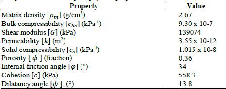
This section presents the analysis of the sand-production test performed to validate the proposed model. The sand-production test was performed on a hollow-cylinder sample, which was made from a mixture of water, sand, and cement [18]. The sample had external and internal diameters of 125 and 25.4 mm, respectively. Table 1 lists the mechanical and petrophysical properties.
During this test, the axial and radial stresses were independently controlled, and the sample was subjected to a pressure gradient to induce a high fluid velocity. The fluid flowed from the external radius to the internal radius. The pressure in the internal diameter was constant and equal to the atmospheric pressure, whereas that in the external diameter was varied. The produced fluid and sand were quantified over the duration of the entire test. Fig. 3 shows the results recorded during the test, which included the pressure drop between the external and internal radii, applied axial and radial stresses, amount of produced sand, and axial deformation of the sample.
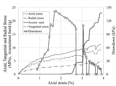
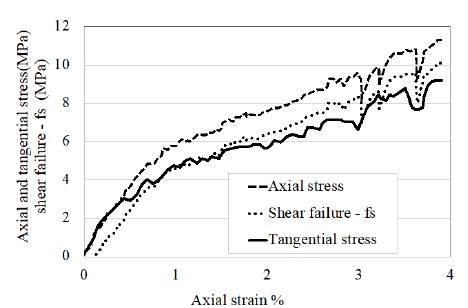
As part of this work, Fig. 3 shows the tangential stress at the inner diameter of the sample. In this case, the tangential stress was calculated at the internal radius of the sample by assuming that the material elastically behaved. This condition considered that σ r inn = 101 kPa, where σ r inn is the radial stress in the internal radius during the test.
To study the sand-production behavior during the test, the sand-production data were divided into four stages (E1, E2, E3, and E4). Each stage had initial and stabilized values of the sand-mass product, as shown in Fig. 4.
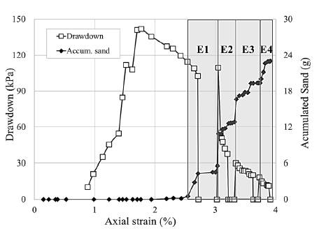
Source: Nouri et al., 2006.
Figure 4 Stages of sand production according to the behavior of the accumulated sand production.
On the basis of our calculation of the tangential stress, the stresses in the inner diameter satisfied the condition that σ v > σ θ int > σ r int , where σ v is the vertical stress, σ θ int is the calculated internal tangential stress, and o r int is the internal radial stress. Using these stresses, we evaluated the Mohr-Coulomb failure function (f s ), i.e., eq. (7) in the inner diameter of the sample (using the data listed in Table 1, namely, pore pressure of 0.1 MPa and Biot coefficient of 1.0). The calculated Mohr-Coulomb failure function (f s ) is shown in Fig. 5. On the basis of the plasticity theory, the failure function cannot have positive values (only negative or zero). However, in this case, this function contained positive values because we evaluated it using the calculated stresses for a totally elastic-material behavior (not plastic). In this manner, the positive values of the f s function indicated that the material exhibited plastic behavior.
Source: own elaboration.
Figure 5 Calculus of the failure function in the internal face of the sample.
In Fig. 5 the plastic behavior started very early in the test, and the sample then accumulated plastic strains and extended the plastic radius, causing in intense material disaggregation in the inner diameter and sand production when the fluid flowed transporting the disaggregated solids.
Fig. 6 shows the relationship between the accumulated sand production with the calculated failure function and the measured pressure drop in the four stages of sand production. Fig. 6 shows that regardless of the behavior of the pressure drop across the sample, a strong relationship existed between the amount of produced sand and the calculated failure function; however, no clear relationship existed between the pressure drop and accumulated sanding response. This condition indicated that the increase in the produced sand was associated with the increase in mechanical loading. This assertion indicated that for real-field applications with sanding events, efforts should be focused on determining the loading state of the formation by knowing the real stress path of the different operations, including those involving temperature changes.
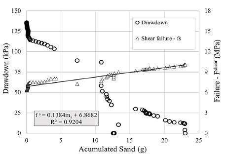
In contrast to the failure-function calculations shown in Fig. 5, the proposed numerical model calculated the plastic strains such that f s = 0 and f s = 0, which was the reason for the use of plastic strains to correlate the production of sand (instead of function f s , as shown in Fig. 6 ). In addition, this condition also explained the definition of a plastic-strain indicator for the sanding-rate criteria. As previously stated, we argued that the sand production in this test was a phenomenon that largely depended on the level of failure of the material near the internal cavity, whereas the moving fluid was responsible for transporting the released grains.
6. Results
6.1 Sand-production modeling
The experimental sand-production test is simulated using the proposed model. The simulated physical model is discretized using 10, 10, and 40 elements in the axial, tangential, and radial directions, respectively. The shape of the modeling elements is a section of a hollow circumference with a height of Δz. The discretization in radial direction is fine enough to get small variations in the calculated variables. In addition, a logarithmic radial discretization is used to obtain finer elements near the inner radius where larger changes in pressure and displacements occur. Table 2 lists the initial conditions for modeling, and the parameters described in Table 1 represent the properties of the base case for modeling. Table 3 lists the fluid properties for simulation.
Table 2 Initial condition and discretization parameters.
| Initial pressure (MPa) | 0.1 |
|---|---|
| Radial, tangential and axial stresses (MPa) | 0.1 |
| Blocks in radial, tangential and axial directions | 40, 10, 10 |
| Block thickness in axial direction [Δz] (m) | 0.025 |
Source: own elaboration.
Table 3 Fluid properties for simulation.
| Property | Value |
|---|---|
| Fluid density [pf] (g/cm3) | 1.0 |
| Fluid viscosity [μ] (cP) | 1.0 |
| Fluid compressibility [c f ] (kPa-1) | 5.80 x 10⁻⁷ |
Source: own elaboration.
Fig. 7 shows the applied boundary conditions. At the top of the model, a displacement boundary condition is applied, thus the axial stress is a simulation result. At the internal radius, the radial stress and pressure are equal to atmospheric (0.1 MPa); at the external radius, the radial stress and pressure are equal to the experimental test data. Non-flow condition is used at the top and bottom faces.
The base case uses the basic parameters for the sand-test modeling as well as the initial and boundary conditions (Fig. 7 and Tables 2 and 3). The axial stress is used to compare and adjust the model results with the experimental results.
The model results for the base and elastic cases are shown in Fig. 8. For the elastic case, the plasticity module is deactivated so that the plastic strains are zero. Comparison of the elastic-case results with real data reveals two scenarios or regions within the test. The first region occurs when the axial strains are lower than 1%. Here the model reproduces the experimental data, and the mean relative error is around 5.2%. The second scenario occurs for axial strains greater than 1% where the simulated axial stresses overestimate the reported experimental results. This result reflects the limitation of the elastic model in representing the stress-strain behavior in highly complex processes where elastic behavior is not the dominant effect and a marked behavior of plasticity exists on the sample.
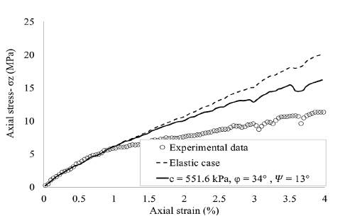
As presented, the reported base-case results demonstrate that the simulated rock appears to have a greater resistance than a real rock, which implies that the real rock loses its initial-strength properties during the plastic-deformation process. This result indicates that constant calibration of the constitutive-model parameters for field operations is critical in predicting the related effects of different operations and procedures over the zones near a wellbore. Therefore, to perform adequate modeling of a real rock, the weakening of the material must be taken into account.
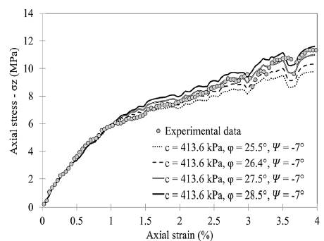
To achieve the best fit between the simulated and recorded test results, a systematic process matching is performed using cohesion c, internal friction angle 𝜑, and dilatation angle 𝛹. This process also facilitates sensitivity analysis of the model, which yields the conclusion that the results are strongly dependent on the internal friction angle, very slightly dependent on the cohesion, and independent of the dilatation. This result emphasizes the importance of accurate determination of the friction angle and model calibration based on the factional angle. Using this methodology for matching parameters, we conclude that the sample also suffers weakening of its strength properties during the test. The best fit is obtained at = 413.7 kPa, 𝜑 = 27.5° and 𝛹 = -7°, for a relative error of 4% (Fig. 9).
6.2 Sand-production adjustment
Regarding the adjustment of the produced amount of sand in the test, the starting point is the adjustment of the stress-strain parameters. Following the same manner in which the correlation between the failure function (on the inner face of the synthetic sample) and sand production is obtained, a correlation between the shear-hardening parameter (e ps ) and experimental data of sand production is obtained by plotting the data of the accumulated sand production against parameter e ps of the test (Fig. 10). A linear correlation is generated for the data in the test, and a remarkable and decisive increase in sand production is verified. From this correlation, the base parameters that control the sand-production function presented in eq. (9) are obtained, namely, μ,A f ,e ps cr , and μ f min .
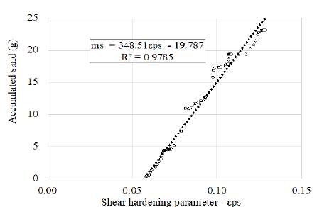
Parameter μ s refers to the slope of the correlation, and parameter e ps cr is the value of the critical shear-hardening parameter that determines the sanding onset. Af is the internal area of the sample, and μ f min is the minimum flow velocity to transport the released sand grains. Parameter μf min is calculated using Darcy's law at the inner face of the sample. Table 4 lists the values of the mentioned parameters.
Table 4 Parameters of the sand-production module.
| Property | Value |
|---|---|
| μs (kg/s) | 0.348 |
| A f (m2) | 0.020 |
| eps cr(adim) | 0.056 |
| μfmin (m/s) | 0.00227 |
Source: own elaboration.
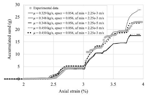
The values of the base parameters associated with the sand-production function are the starting set of the calculation and adjustment of the calculated data of the sand production, which are compared with the data recorded during the laboratory test. In the adjustment process, a sensitivity analysis of parameters μ s and μ f min is performed, which is demonstrated to significantly affect the different characteristics of the curve. Fig. 11 shows the results of the adjustment between the calculated sand production and actual production. The best adjustment is achieved with an error of 3% in the accumulated sand production at the following set of parameters: μ s = 0.45 kg/s, e ps cr = 0.056, μ f min = 0.00225 m/s, and A f = 0.020 m2.
6.3 Sand-production prediction
To verify the model behavior and based on the parameters and adjustment obtained for the axial stress and sand production against the actual sanding test, a sand-production forecast exercise is carried out. This forecast starts at the end of the real sand-production test (axial strain of 4%, see Fig. 11) and extends up to an axial strain of 5% using the same displacement velocity. Additionally, for comparison purposes, four simulation cases are defined (Table 5) where each case has a different increase rate in the external radial stress (based on the radial stress at an axial strain of 4%- 4654 kPa). In other words, at the end of the forecasting (axial strain of 5%) Cases 1-4 increase their external radial stress by 30%, 18%, 15%, and 8%, respectively. In all cases, the flow through the sample is modeled using the same pressure-drop program, which satisfies the criterion of critical flow velocity for sanding. This pressure-drop program models three stages of radial flow with interbedded stages under a no-flow condition. Fig. 12 shows the pressure-drop and radial stresses programs in each simulation case.
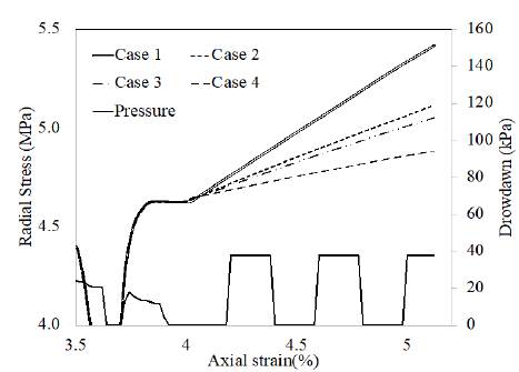
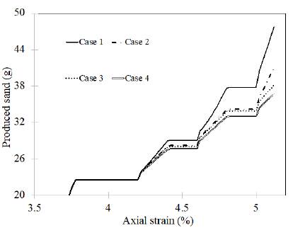
Fig. 13 shows the forecast of sand production for each proposed case. As expected, the level of sand production is a function of the applied radial stress because of the greater concentration of stresses in the inner radius when the external radial stress is increased. In this manner, we can infer that the level of plasticization in Case 1 is more intense than those in the other cases, and this case generates greater sand production. In addition, the sand production is triggered by the fluid flow (sanding does not occur without a fluid flow), whereas the stress-load process (application of vertical displacement and radial stress) generates a constant release of sand. On the other hand, the change from a closed system to a system with a fluid flow (axial strain of 4.25%) generates production of additional sand, which is disaggregated due to the different radial stresses used in each simulation case. This result is reflected in the higher initial slope at the moment when sanding production steps up to an axial strain of 4.25%.
7. Conclusions
According to the laboratory results, using a poroelastic approach, sand production is related to resolving the changes in the yield function using the stress paths associated to the infield processes.
Despite its limitations, the developed model has predicted and quantified the sand production in a laboratory-scale sanding test and requires the adjustment of parameters such as the mechanical properties of a porous medium. Using the proposed model, comparison of the simulated and actual results achieves a relative error of almost 4%, which shows that the elastoplastic constitutive relationships with softening or hardening are essential for modeling weakly consolidated or nonconsolidated formations. In this analysis, the internal friction angle exerts the largest effect on the plastic behavior of the material, followed by cohesion and finally by the dilatation angle, which reflects the great significance of the friction angle in the sand-production predictions.
The elastic constitutive relationships are strongly limited when the behavior of sanding prone formations is modeled. However, the elastoplastic constitutive relationships are more adequate as long as good parameter determination is performed. In addition, modeling of the softening or hardening phenomenon is essential to achieve more coherence and representativeness of the results. This work demonstrates that the strength weakening that occurs in the triaxial tests also occurs in the hollow-cylinder test. This result should be considered in near-wellbore regions because the strength parameters decrease compared with their initial values during the production time and operating procedures.
A sand-production study is carried out, which considers different load-stress and fluid-flow schemes for a real-life experimental test. We find that sand production is directly affected by the level of applied radial stress. Further, this study finds that opening and closing the flow causes an increase in the level of produced sand, similar to the sanding cases found in cyclical injecting or producing wells where the production rate is stopped several times.
Finally, the application of this model in a field case enables quantification of the sanding level and understanding of the main mechanisms from a phenomenological perspective. Moreover, this model can help in accurately predicting possible events and avoiding them especially for unconsolidated or weakly consolidated formations.
This model fully couples fluid flow, geomechanical and sanding models, which allows not only the prediction of sanding onset but also sand quantification. The interaction enabled by this model between the different variables and phenomena is essential for correct management of the production rate and pressure in a wellbore if sanding is completely undesired or for proper design of a completion tool to control sand production.