1. Introduction

Two of the most common intelligent controllers, fuzzy systems and Neural Networks, aims to capture the human capacity to make decisions in an algorithm. Those controllers overcome problems such as losing attention, the frequent necessity of resting, or ethical issues if a human is inside a control loop [¹]. Even when the application of intelligent controllers covers a variety of areas, the advances in computation, and their increasing popularity, intelligent controllers have limitations. This paper proposes a solution to two of the main limitations. The first limitation resides in the time constraints when a human generates the data to train a Neural Network, for instance the applications in [²,³]. The second limitation regards the strong assumption in fuzzy logic about the ability of the expert to express the knowledge in written statements, as shown in [⁴-⁶], which may not be true. We present a proposal to solve those two problems in a single algorithm called Time Scaling Control.

Neural Networks have been successfully used in control application because they emulate human decisions, and we have been controlling everything around us since we have been here, starting with our own bodies. For instance, the simple reach-to-grasp behavior has been demonstrated to be optimal [⁷] and can be used to train robots to make them to have human-like motion in applications that require interaction between robots and humans. Most of the efforts to scientifically measure the human capacity to control, as [⁸], are highly mathematical, which make them useful to prove what everybody knows by intuition, and in addition to measure the limits of our capacities, for instance the frequency response or the latency [⁹]. One of the main limitations of humans to control regards the speed [¹⁰], if the speed is too high we cannot give a proper response, because the brain takes time to make decisions and the muscles also require time to respond, however if the speed of the motion is lower than a certain bound, we also lost the ability to control [¹¹]. Some studies propose methods to improve this speed limitations, for instance to preview the reference or to show predictions of the current behavior [¹²], but the speed barrier remains in place. This paper proposes a method to overcome the speed problem by changing the time scale of the system under control, which solves the first limitation mentioned in the previous paragraph.

There are some proposals to avoid the difficulty that may appear when an expert translates knowledge into writing statements. For instance, the work in [¹³] uses direct signals from the brain to grasp and lift an object using a robot. In addition to the signal acquisition, authors use machine learning to convert the brain signals into a discrete set of commands for the robot. Thus, the human never consciously put the knowledge into a written form. Other authors prefer to use results from studies instead of using the expertise of a single person. Then, for instance, the actions of a person are defined as a set of probabilities which influences the control, as shown in [¹⁴] or [¹⁵]. Another option to avoid the writing of the knowledge consists of using a computer to analyze the data or also using a group of people instead of a single expert, for instance to learn how a person looks for a destination in an unknown environment with obstacles using a simulated environment, in [¹⁶], or the motion of the body to avoid an obstacle, in [¹⁷]. To avoid the writing of the knowledge by an expert we propose to use a Neural Network, but we could use another tool, such as a Support Vector Machine.

This proposal, as well as other techniques in intelligent control, aim to build better controllers by the emulation of a human during a control task. However, and firstly, the author proposes a method to eliminate the limitations caused by the time delay in the brain and body. That delay makes some systems too fast to control, whereas systems that are too slow may cause attention problems. In both cases there may be a reduction in the control performance, which limits the number of dynamic systems that a human can control. Instead, and using the proposal in this paper, a person can control any dynamic system by changing the speed of the system properly.

The intuitive idea of the proposal, called Time Scaling Control (TSC), consists in changing the constant times of a plant until the control is comfortable enough for the human. In general, this is impossible with a real plant, but it is possible with its model. Thus, a person controls a scaled version of the model instead of the real plant. Finally, the knowledge that was captured during the control task is learned by a Neural Network. An important feature of some Neural Network architectures, such as a Multilayer Perceptron, is that they are blind to changes in the time scale so they can be equally used for the scaled model and for the real plant.

The author compares the performance of a fuzzy logic controller, a piecewise linear controller and a TSC for the control of the angular position of a shaft using a DC motor. Following Section presents a central procedure in the controller design, it is the identification of the plant. The next three sections show the steps to design the proposed controller: The Scaling (S), the Training (T), and the Running of the controller (R). The paper continuous with experimental evidence and performance comparisons among the three controllers, and ends with conclusions and future work.

2. Plant description

Time Scaling Control can be applied to any dynamic system, but its advantages become evident when the system is too fast or too slow for a human to control in real time. Thus, the author chose a fast system in this paper, it is the angular position control using a DC motor. In this plant, an input voltage produces a current in the armature winding, which interacts with the field coming from two permanent magnets. The result is a torque that makes the shaft of the motor to rotate. That rotation is counteracted by the friction in the bearings and the inertia of the machine. In terms of modeling the machine has three parts: 1) an electric circuit, 2) an electromechanical part, and 3) a mechanical component. The first part is considered linear when the motor is working near nominal voltage and current, same estimation for the second part, but the mechanical component includes nonlinear aspects, such as saturation, friction, and asymmetries due to the rotation sense.

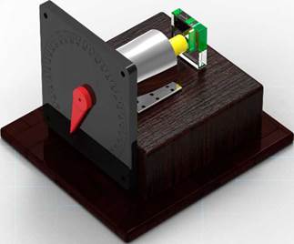
Controlling the motor requires sensing the angular position of the shaft, because the controller constantly compensates any deviation from an ideal position, given by a reference. The most common choice for that sensor is an incremental encoder, due to the low cost and its easy set-up, however a magnetic sensor is used, because it provides absolute measurements instead of discrete values. In addition, the plant includes a protractor and a needle, as shown in Fig. 1, to facilitate the visualization of the position of the shaft.

Source: The author.

Figure 1 Prototype.  

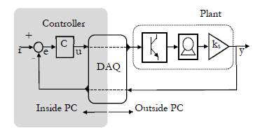
In addition to the motor and the sensors, the plant requires a power amplifier. This stage transforms the actuating signal coming from the controller (implemented inside a computer) into a proportional signal that moves the motor. The connection between the control algorithm and the power amplifier is a Data Acquisition Card (DAQ), which in addition receives the signal from the sensor, as shown in Fig. 2.

Source: The author.

Figure 2 Control scheme.  

The identification of the plant in this paper does not look an exactly accurate model, but a model that captures the key features of the dynamic, because that proved to be enough using Time Scaling Control. The core of the model, presented in the Fig. 3, emulates the transient behavior of the motor using two linear blocks: 1) the relation between the input voltage and the speed in the shaft, and 2) the relation between speed and angular position. Given the authors' experience controlling the motor, there are two main nonlinearities that should be included in its model: 1) the dead zone, and 2) the gain for the steady-state as a function of the rotation sense. The dead zone is represented by the first block in Fig. 3, while the gains correspond to the triangles. The model includes another nonlinearity, the saturation of the integrator, which expresses the natural limits for the rotation of the motor. The block between the gains and the integrator symbolizes the selection of one gain or the other depending on the sense of rotation.

Source: The author.

Figure 3 Block diagram of the motor model. 

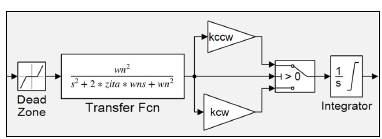
This is the list of parameters for the model in Fig. 3: Dead zone: start of dead zone, sdz, end of the dead zone, edz.

Transient: natural frequency, ω _n , damping ratio, 𝜁. Gains: counterclockwise sense, k _ccw , clockwise sense, k _cw

Saturation: Upper saturation limit, ul, lower saturation limit, 𝑙𝑙.

We start by defining ul and 𝑙𝑙. Even when the control rank equals ±90°, the limits are larger than that. A first extra 10° allows the human controller to make mistakes at the ends of the rank and still generate data to train the controller. A second extra 10° bounds the parameter estimation algorithm in Matlab to vary the parameters of the model. Thus, ul = 110° and 𝑙𝑙 = -110°. The next two parameters correspond to the transfer function, H(s), it is { and u> _n . A method to evaluate them implies generating sudden changes in the input of the motor and then measuring the speed in the shaft. The values that match the transients better are ω _n = 100 rad/s, and 𝜁 = 1.

The four remaining parameters of the model were computed using the tool Parameter Estimation of Simulink. Given that the main goal of the model is to emulate the system when the controller is working, then a proportional controller with k _p = 1 / 10 leads the motor during the acquisition of the input and output data. The whole experiment lasts a minute and uses samples every millisecond. The reference for the control system is a step function randomly changing every 0.3 to 0.7 s with also random amplitude from -90° to 90°. This signal was smoothed using a first order filter with constant time of 0.1 s to emulate the work of the motor during normal conditions. The optimization method is the Nonlinear Least Squares and the algorithm is Levenberg-Marquardt. The tolerance in the optimization is 0.001. A final estimation was run including all the parameters except the saturation constants. As a result, the natural frequency changes to ω _n = 300 rad/s. It is important to report that the change from 100 to 300 in ω _n does not change more that 0.1% the quality of the model, which means that the nonlinearities affect the dynamic of the motor more than the linear part. In summary, the model has the following parameters: dead zone sdz = -0.9, edz = 0.6; transient ω _n = 300, 𝜁 = 1; gains k _cw = 940, k _ccw = 530; and saturation ul = 110°, 𝑙𝑙 = -110°.

2.1 Scaling stage (S)

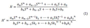
The model in Fig. 3 uses the traditional definition of time, but that dynamic is too fast to control given the human reaction time. Thus, this section starts by scaling the linear components of the motor, as defined in eq. (1), according to the presentation in [¹⁸]. The scaling requires the definition of the scaling factor, k _t . Thus, for instance, if k _t = 2 the new dynamic H' is two times faster than the dynamic H. The new plant, H', keeps amplitude and shape of the model and only changes the transient length. On the other hand, the nonlinear components of the model remain equal regardless the time definition because they are constants.

Defining the scaling factor requires an experimental procedure. In this process, the human changes k _t until the transitions in the experiment can be comfortably controlled. The result for this paper is that k _t = 1/30. Thus, a minute in the experiment equals 2 s in the original scale of time. As a result, the linear component H = 300²/(5² + 6005 + 300²) corresponds to H' = 100/(5 ² + 205 + 100), and the integral θ(s)/Vel(s) = 1/S equals θ’(s)/Vel' (s) = (1/30)/5. In addition, the scaling process requires changing the sampling time at which data is recorded, from t _s to t' _s = t _s /k _t . In this case t _s = 1 ms so t' _s = 30 ms.

Time Scaling Control requires interaction between the human and the scaled system to learn how the human controls. Traditional control uses the error signal (e = r - y) as input to compute the best actuating signal, but TSC uses -e' , as shown in Fig. 4. The use of -e' makes the control action intuitive for a human: it is to counter act the signal in the screen to have null error. For instance, if -e' is negative, a good control action consists in setting u' as a positive value, which eventually increases the output y' , decreasing the error. This counter action control strategy finds its inspiration in the vestibulo-ocular reflex (VOR) which allow humans for instance to read inside a vehicle in motion due to the image stabilization feature [¹⁹].

Source: The author.

Figure 4 Control scheme.  

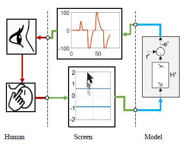
A human, as well as any other controller, makes one of three decisions: to keep the actuating signal, to increase it, or to decrease it because of what happens in the plant. In addition, the controller makes two things: first, decides how large the change is, and second, monitors the system to decide when to make a change according to the effect of previous decisions. That knowledge may not be conscious for a human, and a person may not be able to verbalize it, however the practice makes the brain to make better decisions. TSC takes advantage of the human ability to learn and places that knowledge in an automatic controller.

An automatic controller replaces Human and Screen sections in Fig. 4, defining the actuating signal, u' , to lead the error, e' , toward zero. The remaining section in Fig. 4, the Model, represents the scaled version of the motor as presented in detail in Fig. 5. In that figure the reference was defined as a square signal oscillating between 100° and -100° lasting in each value between 13 to 17 seconds. The experiment lasts 2.5 minutes. Thus, every reference value appears about five times, which is enough data to train the Neural Network in the next stage of the control process.

Source: The author.

Figure 5 Control system in Simulink.  

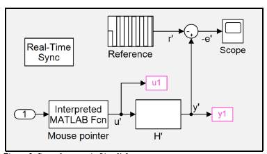
Another block in Fig. 5, "Mouse pointer", captures the mouse position in the screen based on the function "gpos" of Matlab. The "y" coordinate of the pointer corresponds to the u' signal. The blocks "ul" and "yl" in Fig. 5 record the data generated during the simulation and make it available for use in the workspace of Matlab. The signal "ul" corresponds to the actions of the human controller, while "yl" provides the corresponding emulated position given the scaled model. Finally, the block "Real-Time Sync" allows the running of the simulation in real time using the toolbox Simulink Desktop Real-Time, which sets the sampling time at t' _s .

2.2 Training stage (T)

This stage uses the data coming from the human during the control process to train a Neural Network. That Neural Network replaces the human and autonomously controls the motor from that moment on. However, the data is normalized before the training, which implies cutting and scaling. The first 15 seconds of the experiment are deleted because that is the time that a person needs to be accommodated in a right position and to be focus once the simulation starts. On the other hand, the scaling consists in dividing e' by 180, as shown in the horizontal axis in Fig. 6. The scaling is a standard procedure in the training of Neural Networks, given that it facilitates the computation of the connection weights.

Source: The author.

Figure 6 Effect of the number of neurons in the training.  

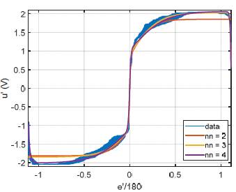
An analysis of the sorted data in Fig. 6 shows the relationship between the error and the actuating signal. That relation makes evident the control strategy of the human, which was hidden inside the brain until now. The control strategy looks like a tangent sigmoid but enlarged by the effect of the dead zone. This observation favors the use of a Multilayer Perceptron Neural Network to learn the data given that each of its neurons may have a tangent sigmoid transfer function.

We can analyze the behavior in Fig. 6 looking for only positive errors given the asymmetry of the figure. That region can be subdivided in four zones. 1) A fast increment: between 0 and 0.1; 2) A smooth behavior: from 0.1 to 0.5; 3) A saturation part: from 0.5 to 1; and 4) A fast decreasing: if the input is larger than 1. The first zone shows how the human avoids the dead zone by feeding the system with a voltage slightly larger the threshold of the dead zone. This zone can be represented using a line with high slope (m ~ 1/0.1). In contrast, the third zone has almost null slope (m ~ 0), because the human counteracts any input larger than 0.5 with the maximum actuating signal possible. The second zone joints first and third zone using a curve, which demonstrates the nonlinearity of the brain decisions. Errors larger than 1 (180°) happen when the motor points down to -90° and the reference suddenly changes to the other end (90°). In this case the human correction lags some fractions of a second. This effect, contrary to the intuition, proved to be useful to decrease the overshoot caused by fast and big transitions.

Authors used the Levenberg-Marquardt algorithm to train the Neural Network and divided the data randomly in three sets: 70% to train, 15% to validate the training, and 15% to test. Results in Fig. 6 regard a Neural Network with a single hidden layer with two, three, and four neurons. Two neurons miss both saturation zones, as shown in Fig. 6. Three neurons match better positive inputs but not the negatives. Four neurons match the whole behavior, which show the simplicity of the human actions to control the system. At the same time, the behavior in Fig. 6 shows the generalization capabilities of a Neural Network, because instead of a fuzzy or cloudy region from the human the Network provides a smooth actuating signal, which improves the stability.

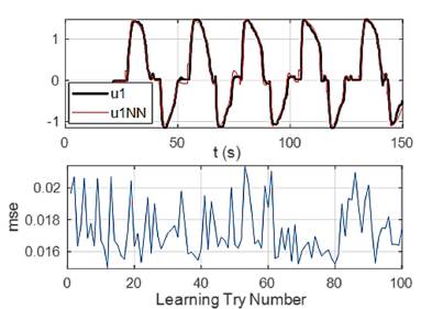
On the other hand, Fig. 7 shows the performance of 100 Neural Networks with four neurons in the hidden layer. The upper part of the figure presents the actuating signal of the Network with the best performance (ulNN) in contrast with the actuating signal of the human (ul). The network closely follows the human control behavior, especially in the zones 2, 3, and 4. The lower part of the figure shows the final mean square error (mse) for each training. This error was used as a measure of quality during the learning process. The variation of mse is not big: the best mse is 0.015, while the worst is 0.022.

Source: The author.

Figure 7 Selection of the best Neural Network.  

2.3 Running stage (R)

This final stage in the control using time scaling uses the best Neural Network of the previous stage. That best Neural Network defines the actuating signal (instead of a human), based on the error value to control both model (at time t') and motor itself (at time t). The reason for this versatility is that a Multilayer Perceptron Neural Network is blind to changes in the scale of time. This type of Neural Network produces the same outputs given the same inputs, regardless of the time variation. If an input changes, the corresponding output is updated after few math operations. These operations are instantaneous in practice given the speed of the systems in contrast with the time to propagate a network. Thus, the same network controls the simulated system and the real plant.

Testing the trained Neural Network starts with running the control over the scaled model, H', because the controller was trained using data from H'. The test during the scaling stage lasts 2.5 minutes because that time is enough to train the network. However, the simulation in this stage may last longer, for instance 30 minutes or more. There is no risk that the Neural Network loses the attention as happens with the human after few minutes. In addition, instead of two unique values ±100°, it is better to test several and random amplitudes in the rank ±90°. If the control works properly, the next step in the testing consists in using the same network over the system H. This last simulation could take a single minute, because the system runs at its normal speed (remember that a minute at the unscaled time corresponds to 30 minutes using the scaled time, kt = 1/30).Thus, the transitions between one amplitude and another may last something between 0.3 to 0.6 s.

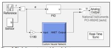
The final and definite test uses the trained Neural Network to control the real plant. The block diagram of the connections inside the computer is shown in Fig. 8. The input of the network is scaled dividing the error by a constant equal to 180. The output of the controller reaches the plant using a data acquisition card, the National Instruments PCI-6024E. This card translates the actuating signal inside the computer into voltages to feed the power amplifier which drives the motor.

Source: The author.

Figure 8 Block diagram to control the real plant.  

3. Fuzzy and linear controllers

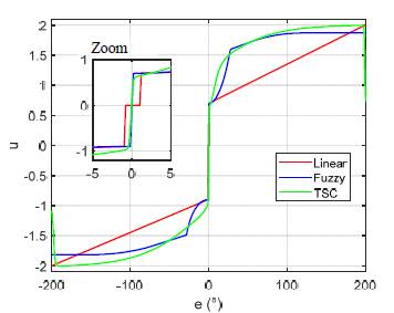
Time Scaling Control, as well as other control strategies such as fuzzy logic control, aims to extract knowledge from a human to control a dynamic system. Thus, this section defines a fuzzy logic controller to contrast the control performance of both controllers. In addition to TSC and Fuzzy Logic we define a third controller: a piecewise linear controller which may resemble an improved proportional controller. This third controller uses heuristics to set the coordinates of each line, as shown in Fig. 10. For instance, maximum and minimum correspond to the limits for the electronic interphase, and initial bounds of 0.7 and -0.9 correspond to the values to overcome the dead zone of the motor; lastly, its actuating signal is zero from -2° to 2° to avoid oscillations in the system response.

Source: The author.

Figure 9 Fuzzy sets.  

Source: The author.

Figure 10 Control surfaces for three controllers. 

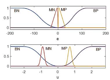
Fuzzy logic has been widely used in the control of dynamic systems during the last years [²⁰]. Given its popularity, this section presents the definition of the input and output sets without detailing concepts of fuzzy control. We define a Mandani type controller with four input sets, as shown in Fig. 9. "BN" stands for Big Negative, whereas "MN" for Medium Negative; MP and BP are the correspondent positive sets. The input is the error "e", defined as the difference between the reference signal "r" and the feedback signal coming from the sensor. The labels for the output sets follow the description done for the inputs, thus for instance "BP" stands for a Big Positive output.

A big positive error in the system happens when the reference is big positive and the angular position is big negative, for instance 90° and -90°, respectively. The best decision for that condition is to set a big positive actuating signal. Following the same logic for the other sets, we define four rules, as shown in the Appendix 1. The combination of input and output sets given by the rules defines the output or control surface, as shown in Fig. 10.

4. Experimental results

The evaluation of a controller requires experimental evidence to measure two aspects: its effort to control and its effectiveness. A traditional experiment looks at the response of the system under sudden changes in the reference, given that this is the harder transition possible. Thus, we designed two experiments using this type of transition, the first experiment makes the motor to start in certain angular position and then the reference suddenly changes to a destination equal to the negative of the origin. The origins go from -90° to 90°, varying every degree, so there are 181 tests per experiment. The second experiment tries every single combination of origins and destinations changing from -90° to 90°, varying every 5°, so there are 1.369 tests per experiment.

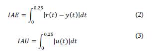
Instead of looking and analyzing the whole transient in each test, we compact the behavior of the system during a test into a single number called performance index. The index IAE (Integral Absolute Error, as defined in eq. (2)), measures the effectiveness of the controller, whereas the index IAU (in eq. (3)) measures the effort of the controller to lead the plant. IAE value indicates the difference between reference and output, whereas IAU value is proportional to the energy used to move the plant by means of the actuating signal u. Thus, a better controller produces smaller indexes. The traditional upper limit for the integrals in eq. (2)-(3) is infinity but given that a normal transient last about 0.15 5, then we consider 0.25 s as the limit of the integral.

A difficulty when running experiments with a real plant consists in the effect of non-modeled characteristics and the appearance of disturbances, for instance the effect of the temperature or the random influence of the friction. Thus, and to decrease those effects the author designed a procedure to guarantee similar conditions in every experiment. In this procedure, the motor is fed with 1.45 V for 10 s and then with -1.75 V for another 10 s; this process is repeated until the rotation in each sense reaches at least 30 x 10 ³ degress (at the average speed of 500 rpm). If the motor is cold, reaching its nominal temperature could mean repeating the process about fifteen times, and about three times when the process is run during the experiment. The voltage, time, and angular position values were defined experimentally and completely depends on the plant.

Fig. 11 presents the results for the running of the first experiment seven hundred times. It was necessary to run this number of experiments because the variations from one running to another given that we are working with a real plant. Only when we aggregate that number of experiments the average of them makes the behavior of the controller evident. IAE performance index is symmetric for TSC at the cost that IAU is larger when the origin is positive, which shows that the human compensates the effect of having different gains depending on the rotation sense. That nonlinearity for IAU is larger in the case of the fuzzy controller, so much that the IAE value is smaller for positive origins than for negative origins. IAE value for the linear controller is the highest, as expected, because the actuating signal is smaller than the other two controllers for every error. Another conclusion from Fig. 11 regards the performance of the controllers at small errors, TSC has the biggest advantage in that region simultaneously having the same effort to control than the other two controllers in that region. Being the best controller remains true for the whole rank of origins, but the biggest difference happens at small errors.

Source: The author.

Figure 11 Control performance comparison. 

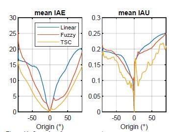
TSC has the lowest IAE performance index with the lowest IAU, so it is the best controller, but it is important to mention that the quality of TSC completely depends on the human during the scaling and training stages, and this also happens with the quality of the fuzzy controller, which depends on the ability of the expert to define sets and rules. Thus, in principle it is possible to find a fuzzy controller that reaches TSC performance or even overpass it, at the same time, in principle it is possible to find another person that after enough training could make the indexes decrease even more than the values in Fig. 11.

In the second experiment, we make a square grid of all origins and destination in the rank of the plant, it is ±90°. The origin starts in -90°, and then runs for all the destinations, then the origin increases 5°, and we repeat the process until the last origin at 90°. Before starting a new origin, we run the procedure to guarantee nominal conditions as it was described before. Thus, this experiment implies 1.369 combinations origin-destination. On the other hand, if the origin equals the destination, the index equals zero because the system starts already in the destination. Given the time to run this experiment we run it only fifteen times and then compute the averages as presented in Figs. 12, 13.

Source: The author.

Figure 12 IAE performance values for the three controllers. 

Source: The author.

Figure 13 IAU performance values for the three controllers. 

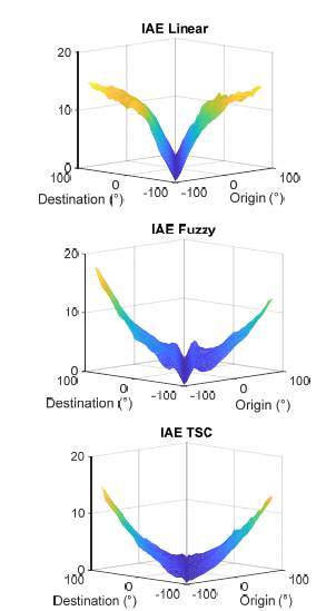
All surfaces in Fig. 12 look like various stages during the fly of a bird and indicate the average IAE value for fifteen experiments. The body of the bird, corresponding to the diagonal with origin equal to the destination, touches the floor with null index value. Any other index value is greater than zero because there is always a transient to go from an origin to a destination. The lowest surface, corresponding to the best controller, is the index for TSC, followed by Fuzzy, however this last surface has a high value when the origins are high negative, as was shown in Fig. 11. The surfaces in Fig. 12 have a symmetry around the axis that goes from one end of a wing to the end of the other wing and shows that the setting in the first experiment properly summarizes the behavior for any origin-destination combination.

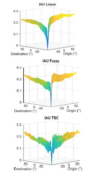
Surfaces in Fig. 13 show the effort of the controller to move the system from the origins to the destinations. All the controllers generate higher actuating signals values when the origin is larger than the destination, in other words for clockwise rotation, as expected, because the gain for that sense is smaller, as found in the model through the values for gains k _cw and k _ccw . Another feature shared by the three controllers regards the magnitude of the index for slight differences between origin and destination, only when origin equals destination the index equals zero, in any other case IAU grows rapidly forming a thin V shape in the performance. The main reason for this behavior is that the controller must break the static friction to make the machine to move and that requires energy.

A feasible way to determine the best controller given the information in Fig. 13 corresponds to sum up all the indexes in each surface. Thus, the best controller has the lowest sum, however it is possible to use any other criterion besides the sum, such as the mean value or the maximum. The sum of IAU reaches 273.6 for the linear controller, 261.1 for the fuzzy controller, and 216.8 for TSC. Thus, in average, TSC uses less effort to control the system. The same sum for IAE produces 10634 for the linear controller, 5888 for the fuzzy controller, and 4484 for TSC. Therefore, TSC is the best controller, followed by the fuzzy controller and the last one in the ranking is the piecewise linear controller.

5. Conclusions

Time Scaling Control changes the time scale of a model to the point that make the actions of a human comfortable enough to control systems otherwise too fast or too slow to control. As an example, this paper presented the control of the angular position of a motor when the model is run thirty times slower than its normal speed. Thus, instead of requiring an expert putting the expertise to control a system in words, as happens in fuzzy control, TSC captures the decisions from the human without conscious intervention to define sets or rules, in addition TSC places that knowledge in an algorithm, such as a Neural Network or any other type of learning algorithm.

The comparison among TSC, fuzzy control, and a piecewise linear controller shows better performance for TSC, followed by the fuzzy controller. A controller is said best if the IAE and IAU indexes are lower that the indexes for its competitors, as it was the case for TSC. However, it is important to remark that the values of those indexes completely depend on some aspects such us the ability of the human to control, so another person could produce better results, at the same time, a better writing of fuzzy sets and rules could result also in better performances for that type of controller.

The main aspects that influence the performance of a human using TSC are three: 1) the time scale gain, 2) the information available in an interphase for the human to control and the interphase itself, and 3) the available time to learn how to control. In this paper, we experimentally optimized the time scale gain, but the other two aspects as well as others that may or may not have influence in the control performance, such as sex or age of the human, are part of future studies to detail the advantages and disadvantages of the use of Time Scaling Control.