


 Inglês (pdf)
 Artigo em XML
 Referências do artigo
 Enviar este artigo por email
 Citado por SciELO
  Citado por Google
  Similares em
SciELO
Similares em
SciELO  Similares em Google
 Permalink
1. Introduction
Paramo is an intertropical ecosystem with dominant scrub vegetation that provides important ecosystem services [1]. This ecosystem is the most important source of water in the Andean highlands [2] and contributes to water storage, flow regulation, and biodiversity [1,3-5]. Ecosystems are very susceptible to changes in land use and climate [6,7]. When such changes occur, the functional capacity and biodiversity of these ecosystems are affected [8]. Afforestation with pine plantations is a common practice in the Ecuador paramo ecosystems [9].Changes in land use from natural grasslands to pine vegetation have several impacts. Flow regime markedly changes, peaks and baseflow are reduced, and water yield decreases owing to higher evapotranspiration [9]. As interception tends to be higher in forests, evaporation from the canopy also increases [10]. Afforestation with pine lowers the total flow [11] and reduces water retention in soils owing to organic carbon matter losses [12,13]. According to Balthazar et al. [14], changing grassland to pine forests is associated with negative impacts, such as a decrease in soil water content, soil organic matter, water retention capacity, and potentially irreversible provision of ecosystem services. Therefore, paramo grasslands must be maintained as pristine as possible. However, in-depth local knowledge on the impact of pine plantations on paramo's hydrology is lacking [9]. Owing to its specific geography, climate, and its hydrologic characteristics, the impact of afforestation on paramo should be significantly different from that on other ecosystems.
Quantifying the effect of land cover change on hydrology requires continuous monitoring over a long period [10,12] before and after the alteration. However, such quantitation is not always feasible. To solve this issue, hydrological models can be used to evaluate land use change scenarios and predict their impacts based on knowledge from other sites [15-18]. A catchment can be modeled with a specific land cover to estimate its parameters [15]. However, the transferal of parameters between catchments to mimic land use changes is a caveat of this model as it has not been fully studied or validated in paramo ecosystems.
This study was carried out to answer the following questions: 1) How can the model parameters in catchments be calibrated to simulate land use change? 2) What is the impact on peaks, total flow, and baseflow when land use changes gradually from tussock grass to pine plantations? 3) What are the differences in the impact of gradual land-use changes from upstream to downstream (U-D) or downstream to upstream (D-U)? The results of this study will allow local governments and key water-related stakeholders to improve their decision-making process for issues related to land use planning, water resources management, and water conservation.
2. Materials
2.1 Study sites
Two paired catchments located in the southern part of Ecuador were selected. The principal catchment is called "Zhurucay," which is divided into 6 sub-catchments (Fig. 1), and Mpinos. Both catchments are typical paramagnetic ecosystems.
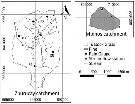
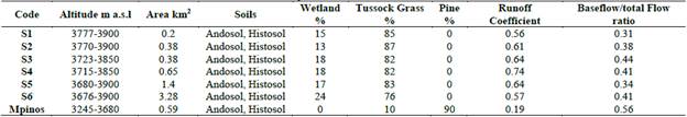
The main catchment characteristics are listed in Table 1. The catchment areas were small, varying between 0.2 and 3.28 km2. Zhurucay is covered by tussock grass while Mpinos is a pine plantation. The elevation for all catchments is between 3245 and 3900 m a.s.l. The soils are the same for all catchments, namely Andosols. The mean temperature is 6.1 °C for the Zhurucay catchment and 8.5 °C for the Mpinos catchment. The average annual precipitation is 1160 mm in Zhurucay and 945 mm in Mpinos. The mean annual runoff is approximately 725 mm for Zhurucay and 180 mm for Mpinos, whereas the average annual baseflow is approximately 280 mm for Zhurucay and 100 mm for Mpinos. The runoff coefficient for the six Zhurucay sub-catchments (S1 to S6) varies from 0.56 to 0.74, whereas that for Mpinos is 0.19. The coefficient was calculated as the observed flow/observed precipitation.
2.2 Data
Despite the size of the catchment areas, precipitation was measured using two tipping-bucket rain gauges at a height of 1.5 m above the soil surface to account for small-scale spatial variability. The resolution of the precipitation was dependent on the type of rain gauge, with values of 0.254 (Onset HOBO Data-Logging Rain Gauge), 0.2 (Davis Instruments Rain Collector II), or 0.1 mm (Texas Electronics Collector Rain Gauge).
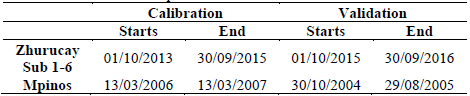
Streamflow was measured at the outlet of each catchment using a compound sharp-crested weir (a triangular-rectangular section was used for high flows, while a V-shaped section was used for low flows) equipped with pressure transducers. Water level was recorded every 5 min. Zhurucay and Mpinos are equipped with a meteorological, station that measures wind speed relative humidity, solar radiation, and temperature at 5-min intervals. There were no gaps in the data for the Zhurucay catchment for the period 01/10/2013 - 30/09/2016 (precipitation, flow, and meteorological variables); however, 16% of the flow data were missing for the period, 30/10/2004 - 13/03/2007, in Mpinos. The available data periods for the calibration and validation are listed in Table 2.
The reference evapotranspiration (ETo) was calculated using the Penman-Monteith equation (1) [19],
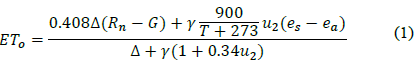
where
ET 0 reference evapotranspiration [mm day-1],
R n net radiation at the crop surface [MJ m-2 day-1],
G soil heat flux density [Mj m-2 day-1],
T mean daily air temperature at 2 m height [°C],
u 2 wind speed at 2 m height [m s-1],
e s saturation vapor pressure [kPa],
e a actual vapor pressure [kPa],
e s - e a saturation vapor pressure deficit [kPa],
Δ slope vapour pressure curve [kPa °C-1],
γpsychometric constant [kPa °C-1].
This method has already been used in Zhurucay and its accuracy was tested by Cordova et al. [20].
2.3 Model conceptualization and description
The HBV-light is a semi-distributed and reservoir-based model that can simulate different vegetation zones, sub-catchments, and hydrological processes based on its routines to compute runoff. The routines used in this study were as follows: 1) the soil routine calculates the recharge to the groundwater and the actual evapotranspiration as a function of water storage for each vegetation zone; 2) the response process transforms the water stored in the reservoirs into runoff; and 3) the routing procedure computes the routing of the runoff at the catchment outlet. More details are provided elsewhere [21].
HBV-light has 11 different structures that vary from one to three reservoirs and possess different spatial distributions according to the vegetation zones. In this study, we used a basic version comprising two reservoirs. The first reservoir is the storage in the upper soil reservoir (SUZ) that receives water from the soil routing and simulates fast flow and interflow (near-surface and subsurface flow). The second reservoir is the storage in the lower soil reservoir (SLZ), which takes water from the first reservoir based on a percolation rate; this reservoir simulates the slow flow (baseflow), as shown in Fig. 2.
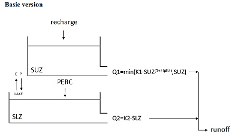
Source: Adapted from Seibert, J., & Vis, M. J. P., 2012
Figure 2 Structure of the HBV-light Basic version of the conceptual model.
We selected the simplest structure to have few parameters that could be related to the hydrological processes mimicking the effect of land use change. This structure was also selected because it has been proven to work well for the Zhurucay catchment [22].
The Zhurucay catchment was divided into six sub-catchments and two vegetation zones, tussock grasses and cushion plants, whereas Mpinos was simulated as a single catchment with pine as the only vegetation.
3. Methodology
Initially, the flow components were separated using the WETSPRO tool [23]. Thereafter, the two catchments were calibrated and validated by applying the split-sample technique. Subsequently, the Monte Carlo (MC) simulation approach was used for calibration, with the Kling-Gupta efficiency (KGE) index and baseflow/total flow ratio as the main objective functions. The calibrated Mpinos parameters were transferred to each of the Zhurucay sub-catchments simulating different land-use change scenarios. Finally, the impacts of these scenarios were evaluated using several statistical indices.
3.1 Sensitivity analysis
The main goal of this analysis was to identify differences in the parameters and their sensitivity between traditional calibration and the baseflow/total flow ratio as an additional objective function approach. A total of 50,000 simulations were performed for the six sub-catchments of the Zhurucay Basin using the MC technique. However, one million simulations were performed for the Mpinos catchment, as 50,000 simulations did not yield enough behavioral sets for the sensitivity analysis. After simulations over 0.4 for KGE and Nash-Sutcliffe efficiency (NSE), were selected as behavioral, each parameter vs. KGE was plotted.
To improve the calibration procedure (with the objective of simulating land use change), we used the baseflow/total flow ratio as an additional objective function; this use not only enables calibration of the total flow, but also the baseflow. The latter improved the sensitivity of the PERC parameter, which controlled the amount of water flowing from the upper reservoir to the second reservoir. The flow was separated using the WETSPRO tool into two components: runoff and baseflow, and the observed baseflow/total flow ratio was calculated for each sub-catchment. Using the same MC simulation results (simulations over 0.4 for KGE and NSE), we applied the baseflow/total flow ratio (with a maximum error of 5%) of the observed and simulated data as an extra objective function and then replotted the graphs.
3.2 Model calibration and validation
Time-series data were separated into two independent periods using the split-sample technique. The calibration and validation periods are listed in Table 2. A longer period for Mpinos was selected for calibration. The first month of the period was copied backward during all simulations as a warm-up period.
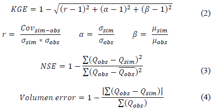
KGE (eq. 2) was used as the main index to evaluate the model calibration performance. The Nash-Sutcliffe model efficiency coefficient (NSE) (Eq. 3) was also used. However, NSE improves its performance by underestimating flow simulations, while KGE does not have this issue, and thereby better representing both high and low flows [24]. The volume errors were calculated using Eq. (4).
To select the best set of parameters, the right baseflow/total flow ratio of the observed and simulated data was considered (the maximum accepted error was 5 %) as the model should not only perform in an ideal manner on the total flow, but also on the sub-components of runoff and baseflow.
Calibration of the Zhurucay sub-catchments was performed using the behavioral sets of the previous analysis (based on the baseflow/total flow ratio); this began with the calibration of the headwater sub-catchments and then moving downstream. First, the S1, S2, and S3 sub-catchments were calibrated to obtain the best-fitting parameters for each catchment. Thereafter, the S4 and S5 sub-catchments were calibrated, followed by the S6 sub-catchment. Calibration of the Mpinos catchment was accomplished using the first 50,000 MC simulations to maintain the same conditions for the calibration of all sub-catchments.
To select the best fitting parameters, the following steps were taken:
50,000 model runs using the MC technique.
For KGE and NSE, the simulations with values over 0.4 KGE and a maximum error of 5% on the baseflow/total flow ratio were selected as behavioral; the remaining simulations were not considered for analysis. For example, for sub-catchment S1, the observed baseflow/total flow ratio is 0.31. Therefore, only simulations with baseflow/total flow ratios of 0.2950.326 were selected. On average 4,000 of the 50,000 simulations were selected for the next step.
Simulations from step 2 were ordered from higher to lower based on KGE values. Thereafter, the top simulation was selected; however, when similar KGE values were found, NSE and volume error were considered to select the best-calibrated model. Validation was performed using the same calibrated parameters for an independent period. KGE, NSE, and volume error were calculated for these periods, and the KGE and NSE values were considered satisfactory for values above 0.5 [25,26].
The following procedure yielded the best fitting parameters to represent the land use of pine in the Mpinos catchment and tussock grass in the Zhurucay sub-catchments.
3.3 Land use change scenarios
The pine land use parameters, derived from the Mpinos calibration, were transferred to each tussock grass sub-catchment of the Zhurucay Basin to mimic land-use change. FC, LP, BETA (vegetation zone parameters), and PERC were the main parameters for transfer as they were controlled by the model land use. FC represents the maximum soil moisture storage (mm), LP is the soil moisture value above which E act reaches E pot (mm), BETA is the parameter that determines the relative contribution to runoff from rain or snowmelt (-), and PERC is the maximum percolation to the lower zone (mm day-1).
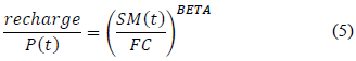
In eq. (5) rainfall (P) is divided into the water filling the soil box and groundwater recharge, depending on the relation between the water content of the soil box (SM [mm]) and FC [mm]). BETA (eq. 5) determines the relative contribution of rain to runoff [27].
LP in eq. (6) is the soil moisture value above which the actual evapotranspiration (E act ) reaches the potential evapotranspiration (E pot ) (mm). Actual evaporation from the soil box equals the potential evaporation if SM/FC is above LP, whereas a linear reduction is used when SM/FC is below LP.
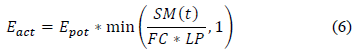
Table 3 Percent change of tussock grasses to pine for the 11 scenarios of land use change
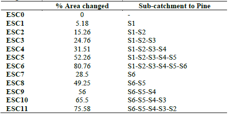
Source: Authors
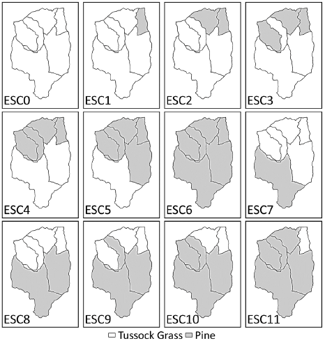
The designed scenarios were a function of the percentage of land use change area (i.e., sub-catchment) and location in the Zhurucay catchment. A total of 11 scenarios were evaluated considering land-use changes from D-U and U-D. The selected scenarios were representative of this region. Scenarios D-U were more likely to occur when the agricultural frontier increased. However, it is easier to begin using land D-U. Of note, afforestation can be used either way. Afforestation with pine is a widespread practice in the Ecuadorian highlands owing to its benefits (e.g., reduced erosion) [9].
The scenarios to be evaluated, the percentage of change, and the sub-catchments that are going to be altered from tussock grass to pine are shown in Table 3, in the same order as shown in Fig. 3. The baseline condition corresponded to ESC0 (80.76% land use with tussock grass).
3.4 Evaluation indices to quantify the effect of land use change and relative error between two approaches (U-D and D-U)
To quantify the effect of land use change, the following indices were applied: runoff coefficient, total flow volume, baseflow volume, average difference in peaks, and FDC (percentiles 10, 50, and 90). The runoff coefficient and total flow volume permit checking the proportion of water yield affected by land use change. The baseflow volume will enable the estimation of how slow flow is affected by land use change, not only during precipitation events but also when no precipitation events occur (i.e., in dry periods). The average difference in peaks, computed as the average of the absolute values of the differences between the peaks of the scenarios and the baseline (ESC0) in percentage, enables the visualization of the impact on high flows (Eq. 7). The relative error between the two approaches (U-D and D-U) permits a quantitative comparison of these options. Finally, the FDC (percentiles 10, 50, and 90) can be used as a measure of the magnitude and frequency of streamflow.
The curves enable a comparison of the complete range of flows and how they might alter under land-use change. Many studies use and recommend using FDC and its percentiles to evaluate the impact of land use/cover change on the different magnitudes of streamflow: (high (P10), medium (P50), and low (P90) flows ([28-32])).
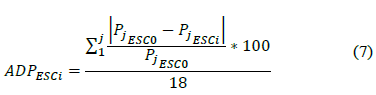
where
ADP ESCi is the average difference in peaks for ESCi
i is the scenario number, goes from 1 to 11
P jESC0 is the value peak for position j of the ESC0
P jESC0 is the value peak for position j of the ESCi
j is the peak number, goes from 1 to 18
4. Results
4.1 Sensitivity Analysis
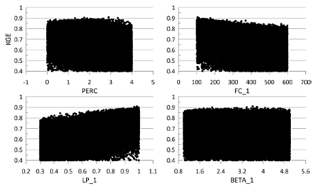
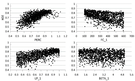
The PERC parameter changes its sensitivity when the baseflow/total flow ratio is used as an objective function, as shown in Fig. 4-7. Only four parameters (PERC, FC_1, LP_1, and BETA_1) that are controlled by land use are shown in this section; the remaining parameters are not sensitive and are not shown here. In the text, only representative figures of the sensitivity analysis (i.e., S1 sub-catchment) are provided.
Source: Authors
Figure 4 S1 sub-catchment sensitivity analysis for the four transferred parameters (traditional calibration).
Source: Authors.
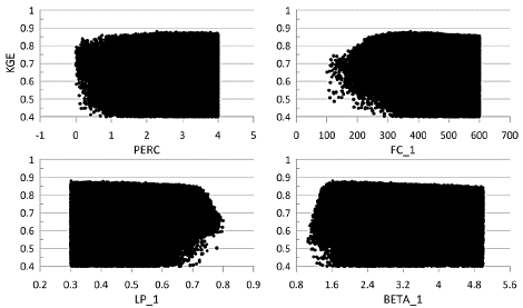
Figure 5 S1 sub-catchment sensitivity analysis for the four transferred parameters (baseflow/total flow ratio included).
Source: Authors
Figure 6 Mpinos catchment sensitivity analysis for the four transferred parameters (traditional calibration).
The S1 sub-catchment sensitivity analysis for the four transferred parameters for traditional calibration is presented in Fig. 4. PERC and BETA_1 revealed no sensitivity, while FC_1 tended to have lower values near 100 and LP_1 to high values close to 1.
Fig. 5 shows the same graph as Fig. 4; however, the baseflow/total flow ratio is included as an objective function. Evidently, FC_1, LP_1, and BETA_1 are similar to those in Fig.4; however, PERC is more sensitive, showing better performance for values between 0.6 and 1.15. Of note, BETA_1 showed no sensitivity. As depicted in Fig. 5, when the baseflow/total flow ratio is used as an objective function, the total number of behavioral simulations is reduced to 3%. Thus, only this small percentage of simulations can properly model both the total flow and baseflow, in contrast to the results shown in Fig. 4.
Source: Authors
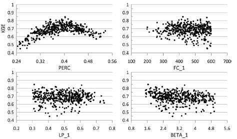
Figure 7 Mpinos sub-catchment sensitivity analysis for the four transferred parameters (baseflow/total flow ratio included).
Fig. 6 presents the sensitivity analysis of the Mpinos catchment for the four transferred parameters. PERC and BETA_1 showed no sensitivity, FC_1 tended to have values above 200, and LP_1 had values between 0.3 and 0.75.
The baseflow/total flow ratio was applied to the Mpinos catchment area in Fig. 7. PERC becomes sensitive, showing an optimal range between 0.33 and 0.42; FC_1 is between 400 and 600 and LP_1 is between 0.3 and 0.62. The optimal values for BETA_1 were between 1.6 and 3.6. When the baseflow/total flow ratio was applied (Fig. 7), the behavioral simulations were only 0.5% of the number of behavioral simulations shown in Fig. 6.
4.2 Calibration and validation
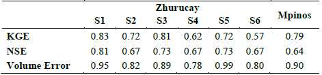
The calculated indices for all sub-catchments are presented in Tables 4 and 5. The KGE, NSE, and volume error values were satisfactory for both the calibration and validation. KGE is always higher than 0.69 for calibration and 0.57 for validation. However, NSE is always higher than 0.57 for calibration and 0.64 for validation.
Table 4 Statistical indices for the calibration period for the land uses of tussock-grass (Zhurucay) and pine plantation (Mpinos).
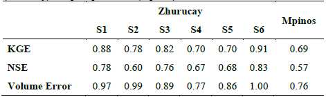
Source: Authors
The model adequately represents rainfall-runoff interactions and the proportion of baseflow/total flow. The average volume error was 11% for calibration and 12% for validation.
Table 5 Statistical indices for the validation period for the land uses of tussock-grass
Source: Authors
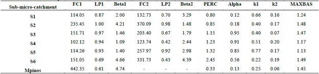
The best model parameters based on 50,000 MC simulations are listed in Table 6. The FC1 parameter for the Zhurucay sub-catchments is, on average, 145, whereas that for Mpinos is 442. Such finding indicates that the maximum soil storage for pine is three times greater than that for tussock grass. The LP 1 parameter for the Zhurucay sub-catchments is, on average, 0.9 while that for Mpinos is 0.6; this will produce more evapotranspiration in the Mpinos catchment. The BeTA1 parameter for the Zhurucay sub-catchments is, on average, 2.47 while that for Mpinos is 4.74. This result indicates that the relative contribution from rain to runoff will be superior for Mpinos. The PERC parameter for the Zhurucay sub-catchments is, on average, 1.3 while that for Mpinos is 0.3, indicating that the maximum percolation to the lower zone will be higher for Zhurucay. These parameters are the main parameters for transfer as they are controlled by land use in the model. As shown, there is a clear difference in the calibrated parameter values between the two catchments owing to the distinct land-use cover.
4.3 Land use change scenarios
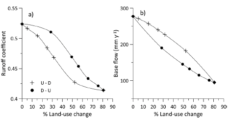
The runoff coefficient decreases from 0.52 to 0.41 (or the total flow decreases from 607 mm/year to 479 mm/year) when 81% of the land cover is changed (ESC 6) from tussock grass to pine, as shown in Fig. 8a; this corresponds to a 20.9% reduction. When land use was changed to D-U, the runoff coefficient (or total flow) was always higher than that of the other options (i.e., from U-D). For example, when 30% of land use changes, the runoff coefficient was 0.51 for the D-U approach and 0.47 for the U-D approach; the difference is approximately 8%.
Source: Authors
Figure 8 Change in the runoff coefficient (a) and baseflow (b) in response to a cumulative land use change from tussock-grass to pine plantation. U-D represents upstream to downstream, and D-U represents downstream to upstream land use change.
The baseflow volume of the Zhurucay catchment was 278 mm/year under current conditions (tussock grass-covered); however, when the land use change to pine was approximately 81% of the area (ESC 6), the volume can be as low as 95 mm/year (Fig. 8b), representing a 66% decline. In contrast to the runoff coefficient, the trend for baseflow was different; baseflow was always lower when land use change was implemented from DU. For example, when 30% of land use was changed, the baseflow was 227 mm/year for the U-D approach and 190 mm/year for the D-U approach, a difference of 13%.
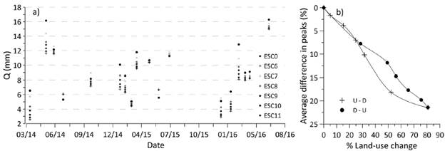
When land use was changed from tussock grass to pine, there was a decrease in the discharge peaks (Fig. 9a) compared with the baseline condition (ESC0). The average difference (decline) in the peaks reached 21.4% when 81% of the area was changed to pine (Fig. 9b). However, this average increased gradually as the land use change area increased. Single differences (decrease in peak discharge) could be as high as 61%. From 0% to 25% land use change, no significant difference was found between the D-U or U-D approaches. Higher percentages of land-use change areas show that the average differences in peaks are always larger for the U-D option. For example, when nearly 50% of land use changes, the average differences in peaks are approximately 18% for the U-D approach and 12% for the DU option, a difference of 6% between both approaches. However, this difference can be as high as 18% (51% for the U-D option and 33% for the D-U option) when the difference in peaks is considered individually.
Source: Authors
Figure 9 Peaks for the different scenarios of the D-U approach (a) and average differences in the peaks (average of the absolute values of the differences between the peaks of the scenarios and the baseline (ESC0) in percent) (b) in response to a cumulative land use change from tussock-grass to pine plantation. U-D represents upstream to downstream, and D-U represents downstream to upstream land use change.
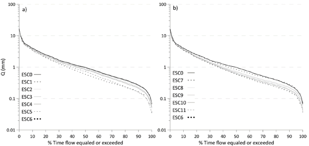
FDC analysis is a common practice for evaluating the impact of land use change on streamflow. Fig. 10 shows that discharge always decreases when land use change increases from tussock grass to pine plantations in both approaches (U-D and D-U). However, the impact was not the same for high, medium, and low flows. For example, between ESC0 and ESC6, reductions of 13%, 40%, and 38% were found for high flows (P10), medium flows (P50), and low flows (P90), respectively. The FDC results show that no evident difference exists between the U-D (Fig. 10a) and D-U (Fig. 10b) options.
Source: Authors.
Figure 10 Flow duration curves for a gradual cumulative land use change from tussock-grass to pine plantation: Upstream to downstream (U-D) land use change (a), Downstream to upstream (D-U) land use change (b).
Table 6 Best sets of model parameters based on 50,000 Monte Carlo simulations for each sub-catchment.
Source: Authors.
Figure 9. Peaks for the different scenarios of the D-U approach (a) and average differences in the peaks (average of the absolute values of the differences between the peaks of the scenarios and the baseline (ESC0) in percent) (b) in response to a cumulative land use change from tussock-grass to pine plantation. U-D represents upstream to downstream, and D-U represents downstream to upstream land use change. Source: Authors
5. Discussion
Based on the results of this study, the model parameters can be properly calibrated to simulate land-use changes. Such calibration was achieved by combining the traditional calibration method with the baseflow to total flow ratio. First, the sensitivity analysis revealed different ranges of values between land uses for three of the four transferred parameters (PERC, FC_1, and LP_1). Of note, the BETA_1 parameter is intimately related to the FC_1 parameter (Eq. 5). Second, the results on the impact of land use change are consistent with those of other studies, such as a decrease in total flow, baseflow, and peaks, and an increase in evapotranspiration (ET) [9,10,12,33,34].
The current study found that almost 21% of the total flow and 66% of the baseflow were reduced after land use change from tussock grass to pine plantation (ESC6: 81 % of land use change) (Fig. 8 a&b). These results corroborate those presented in the literature. For example, Farley et al. analyzed 26 afforestation cases, 13 of which were originally grasslands. The decline in total flow and baseflow might be due to an increase in ET, which is higher in forests than in grasslands [35]; however, a decline in soil moisture is also expected [1,10,12,13].
The reduction in the total flow (21%) in this study was lower than that reported by Buytaert et al. [9], who found a 50% decrease. These differences could be explained by the difference in altitude; the Zhurucay catchment (3676-3900m а. s.l) is situated at a higher altitude than the other study site (2980-3810m a.s.l). Cordova et al. [36] found that for every 1000 m increase in altitude, the temperature decreases by approximately 7 °C, and a lower temperature results in a lower ET, ultimately resulting in higher flows. Farley et al. [10] analyzed 26 afforestation cases and found that the average reduction from mean annual precipitation was 14%; however, in our study, a reduction of 11% was found for similar percentages of land use change area (84% (on average) and 81%, respectively).
Interestingly, the U-D approach had a higher impact on the total flow and peaks (Fig. 8,9) and a higher impact than the D-U approach. These results are contrary to those of Vertessy et al. [37], who found that the D-U approach has a higher impact than the U-D approach based on model predictions. According to these researchers, in higher situated areas, ET is less than that in lower areas. At our study site, there was a small variation in altitude (224 m); this variation was not large enough to evaluate the altitudinal effect on ET. These contradictory findings suggest that a further investigation is needed using experimental data as both studies are based on modeling. In Fig. 8b, the D-U approach has a higher impact than the U-D approach on baseflow. As pine trees consume more water in lower than higher lands owing to altitude differences and the conditions for transpiration, this could explain the results obtained.
Evidently, the impact of FDC is stronger on low flows (P90) than medium (P50) and high flows (P10) (Fig. 10), which agrees with the results of Scott and Smith [38] and Farley et al. Such finding indicates that the impact of land-use change is larger in dry periods than in humid periods. Scott et al. reported that a strong reduction in baseflow is expected after afforestation. This effect might be related to the ability of tree roots to access water deeper in the soil even under dry conditions [39]. Buytaert et al. [9], who employed conditions similar to those in this study (tussock grass and pine plantation), revealed reductions in peaks and baseflow (Fig. 8b,9). Maximum events are absorbed by the pine plantation owing to higher consumption and higher evapotranspiration; however, during no-rainfall events, flow can be reduced to values close to zero for the same reason [29]. Similar FDCs were found for scenarios ESC0 and ESC6 (Fig. 10), with less regulated volume during the application of land-use change.
As stated by Buytaert et al. [33], in the Andean region land use change could be more severe than climate change and is easier to control. As these problems can become critical, effective land use planning might become more stringent than the management of the effects of climate change.
б. Conclusions
Based on the findings of this study, land use change simulation can be implemented by calibrating the parameters of the HBV-light model using the baseflow/total flow ratio in addition to the traditional calibration procedure. Herein, the most relevant parameters related to land use and their sensitivities were identified (i.e., PERC, FC_1, LP_1, and BETA_1). This new understanding should help improve predictions of the impact of land use change from tussock grass to pine plantations on a paramo ecosystem. Further, this calibration procedure can be replicated using different types of land use in the same or different ecosystems. The total flow and baseflow were reduced by 21% and 66%, respectively, and peaks could be reduced by 21%, on average, and individually as high as 61% when land use change was applied from tussock-grass to pine plantations. Of note, the impact was stronger in dry periods than humid periods. The results also suggest that further investigations are needed to correctly define the influence of plantation location (i.e., U-D and D-U) on catchment water balance. Such information could be elucidated using experimental data, which takes many years to collect, or physically distributed models requiring more detailed information for model implementation and calibration. Low flow was found to decrease considerably during pine cultivation. The strong reduction in low flows can cause shortages in the supply of water for human consumption and irrigation, which is a critical issue for water managers. Overall, this study yields a calibration approach that enables the quantification of the effects of land-use change before its implementation. These tools are low-cost and can be used in many applications, such as land use planning, water resource management, and water conservation.

