


 English (pdf)
 Article in xml format
 Article references
 Send this article by e-mail
 Cited by SciELO
  Cited by Google
  Similars in
SciELO
Similars in
SciELO  Similars in Google
 Permalink
1 Introduction
Mass transportation systems have heterogeneous fleets with different types of buses operating on different routes. Each bus is assigned to one of the many workshop yards (WY) which these transportation systems usually have. Every day, each bus must travel empty, i.e., without passengers, from its WY to the starting point of the route, and when this finishes, the bus must return empty to one of the WY. The total distance traveled empty by the bus is known as 'dead kilometers' or 'deadheading', which becomes larger when the buses make more routes and cover major city areas. Deadheading cannot be eliminated, but its reduction may generate important cost savings for transportation operators.
The problem under study in this article can be classified as bus scheduling or allocation to a depot or WY. Problems of this type seek to determine the optimal scheduling or allocation that minimizes the fleet size and operational costs, considering deadheading and waiting times. These problems are known to be NP-hard [1], and several approaches such as Mixed Integer Programming models (MlP), heuristics and metaheuristics, and exact algorithms have been applied to solve them. For example, [1] and [2] apply MIP models to minimize the total distance traveled by buses, considering depot capacities and time periods of operation; these models consider that the initial and final points in a route can be different. In [3], the authors minimize vehicle trips without passengers and the initial and final points in a route can also be different; another work minimizes the fleet size and operational costs by reducing deadheading [4]. A large-scale bus scheduling problem that considers route time constraints is solved in [5]. This formulation decreases the problem size by 40% in comparison to existing models while keeping feasible solutions; the applied heuristics generates near-optimal solutions with maximum gaps of 0.5%.
Some of the research concentrates on genetic algorithms, such as the one developed by [6], who improve the results presented in [7]. Exact methods are applied in [8] to optimize vehicle jobs assigned to several depots to cover a set of scheduled trips. In this case, the vehicle must return to the initial depot and there are constraints on job and total times. In [9], the authors apply a branch integer programming method to optimize the increase of depot capacities and the number of vehicles considering the trips from depots to the initial point of a route. Four models are developed in [10] to minimize dead mileage, differentiating among licensees and considering depot capacities. In this work, the starting and ending points of a job must be the same. Some research addresses the depot location problem and the allocation of buses to depots to minimize dead kilometers and transportation system costs [1-13].
In Colombia, there have been some works that consider deadhead minimization, focusing on bus scheduling. Baldoquin and Rengifo-Campo [14] formulate a multi-objective mixed-integer linear model to solve a vehicle scheduling problem that arises from the mass transportation system MIO in Cali. The authors apply a weighted sum approach with normalization to solve it. Although the authors consider depot capacity, it is given and fixed. They also assume that a bus finishing a task may return to a depot different from the one where it started.
Marin-Moreno et al. [15] concentrate on vehicle scheduling and the algorithms to solve a binary model formulated by the authors. Fuel cost is considered in the objective function because of deadheading. However, no depot capacity analyses are performed because it is given and fixed. Also, a bus can return to a different depot from the one where it started. Therefore, the authors do not analyze the current situation where the bus must return to the same starting depot. The authors apply the model in a real case in Pereira, Colombia, by analyzing the model results on a single working day and for a single bus type.
In this article we considered the mass transportation system in the city of Cali, Colombia. This system operates most routes and buses in the city and comprises a managing company; four licensees that operate the system and own the buses [16]; four WY, each one managed by a different licensee; and more than 4,900 bus stops [17]. On a weekday, more than 1,000 jobs and 898 buses are scheduled. A job is specified by its start and end times, the initial and final stops of the route, and the number of trips to make during the day (see Table 1). A route is the path followed by a bus from an origin to a destination, making different stops along the journey. Several jobs may be scheduled on the same route, but only one bus can perform each job. Since each WY is managed by only one licensee, every day each bus starts a job from the same WY and must return to it when the job has been completed. This means that a licensee does not share the WY that it manages with other licensees. For example, a bus finishing its job in the south of the city may have to travel to its WY located in the north. This leads to the increase in the dead kilometers traveled by the buses, causing additional fuel consumption and vehicle wear, large operating times, increase in variable wage costs, and thus higher operational costs. Currently, the buses travel approximately 17,319 dead km/weekday, generating fuel costs of around 28 million COP$ per day (approximately 7,300 US$ per day).

Deadheading could be reduced by avoiding the situation shown in Fig. 1, where a bus, ending a job at the Universidades stop located in the south of the city, must travel 20.1 km to WY2 to park the vehicle until the next day. If the bus could be parked in WY1, located in the south, it would only have to travel 4.69 km. Certainly, WY capacities must be considered when analyzing these possible improvements.
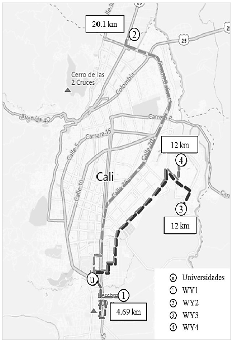
Source: The authors, based on public transportation system information.
Figure 1 A typical trip that generates relevant dead kilometers.
Given the high deadheading costs, we formulate a mathematical optimization model and analyze different scenarios to minimize these costs, such as the impact on the fuel cost if any bus could enter or leave any WY independently of its ownership. We consider the different types of buses, WY parking capacities, hourly demands over a weekday, and the participation of each licensee's WY in the operation. The participation corresponds to the percentage of jobs allocated to each licensee with respect to the total.
Our model focuses on the minimization of fuel costs and considers the following additional issues. Since the fuel cost depends on the kind of bus, dead kilometers should be converted into fuel cost, based on the type of bus assigned to each job. In addition, our model compares fuel costs for the current situation with fuel costs when the depot capacities are changed. In other words, we concentrate on the characteristics of each depot. Finally, our fourth scenario analyzes the distribution of the initial inventory of buses at each depot over five consecutive working days to further minimize fuel costs. Section 2 shows the methodology containing the mathematical model, section 3 presents the results and the analysis of the different scenarios considered, and section 4 concludes the article.
2 Methodology
This section proposes a mathematical model to determine the optimal allocation of buses to WY, including the start and the end of the operation. The objective is to minimize the total daily fuel costs due to the bus trips without passengers. The model includes WY capacities, hourly demands over a weekday, and licensee participation in the operation.
2.1 Assumptions
We assumed the following:
The model only includes fuel consumption costs and ignores other possible costs such as mechanical wear and tear of the vehicle, salary costs and additional costs for increased tire use, and labor and input costs for preventive or corrective maintenance. Therefore, the possible savings from minimizing dead kilometers could be greater than further presented.
Each WY has a fixed location and a limited capacity in the number of buses without considering the specific type of vehicle. This assumption comes from the current observation at a WY in which it is very important to avoid vehicle parking conflicts, interference, and congestion at the parking lot.
The vehicles receive maintenance at the WY without affecting operations.
The base scenario reflects the current system operation in which a bus must return to its starting WY. To optimize, this fact is relaxed in the model, and the ending WY could be different from the starting one. The distance matrix among stops is symmetric, that is, the distance from stop A to stop B is equal to the distance from stop B to stop A.
Each weekday the hours of operation are from 03:00 (defined as period t = 3) to 24:00 midnight (defined as period t = 24).
At the beginning of a day, a list of scheduled jobs is available.
2.2 Notation and mathematical optimization model
For the sake of clarity, the sets, subsets, and parameters are defined in upper case, while decision variables are defined in lower case.
Sets and indexes
WYS: Set of WYs, indexed by i (i = 1, m).
STOP: Set of system stops which are the start or the end of a route, indexed by j (j = 1, ..., n).
PER: Set of one-hour periods, indexed by t (t = 3, ..., T); period 3= 03:00 am, period 24 = midnight= 24:00 = T.
TYPE: Set of bus types, indexed by k (k = 1, ..., K).
Subsets
SS: Set of stops which are the start of a route, indexed by j (j= 1, n).
ES: Set of stops which are the end of a route, indexed by j (j= 1, n).
Parameters
DISTij = Distance from WY i to stop j and vice versa [km].
CAPWYi = Capacity of WY i [Number of buses].
DEMSjkt = Number of type k buses that must start a job at stop j in period t [Number of buses].
DEMEjkt = Number of type k buses that must finish a job at stop j in period t [Number of buses].
EFFICk = Kilometers traveled by type k bus per gallon of fuel [km/gal].
FUEL_C = Cost per gallon of fuel (biodiesel) [COP$/gal].
INVik3 = Number of type k buses parked in WY i at the beginning of period 3 on a weekday [Number of buses]. PARi = Participation percentage of each WY i in the operation.
Decision variables
xijkt = Number of type k buses that travel from WY i to stop j in period t (number of buses that enter the system). yjikt = Number of type k buses that travel from stop j to Wy i in period t (number of buses that leave the system). invikt = Number of type k buses parked in WY i at the end of period t.
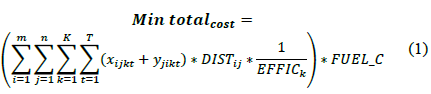
Constraints
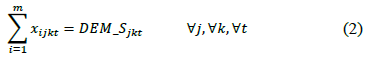
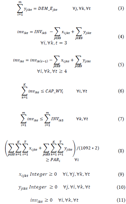
The objective function (1) minimizes total daily fuel costs. Note that this is not equivalent to minimizing dead kilometers because the fuel consumption efficiency in km/gallon is different for each type of bus. Constraints (2) ensure that the buses of each type coming from all WYs, allocated to each starting stop at each one-hour period, are equal to the required vehicles according to the specified hourly demand. Similarly, constraints (3) ensure that the buses of each type arriving at their ending stop at each one-hour period leave the system to some WY selected by the model. (4) and (5) are balance constraints on the number of buses by WY, type of bus, and one-hour period, for the first one-hour period (t = 3) and for subsequent periods (t > 4), respectively. Constraints (6) ensure that the number of buses parked at each WY at the end of each one-hour period does not exceed the capacity of the WY; note that these constraints apply for the sum over all bus types, as mentioned in the model assumptions. Constraints (7) limit the number of vehicles (by type and one-hour period) parked in all WYs to the number of vehicles available at the beginning of the first one-hour period (t = 3). The minimum percentage of participation in the operation of each licensee and its corresponding WY is guaranteed by constraints (8); these constraints consider that the total number of jobs on a weekday is equal to 1,092 and the number of empty trips is thus equal to double the number of jobs. Finally, constraints (9) to (11) are the definition of decision variables.
3 Results and discussion
This section describes the case under study, the results of the proposed model, and three sensitivity analyses. In all cases, the model considers that any vehicle can be parked at any WY, not necessarily the same one where the bus started its job. All cases will be compared with the current operation of the system, where a bus that ends, a job must return to the WY where the vehicle started such job. The four cases are the following:
Case 1: Running the complete model including all constraints from (2) to (11).
Case 2: Running the model without participation constraints (8). Here, the percentage of participation of each licensee in the operation is relaxed.
Case 3 : Redefining capacity constraints (6) by considering additional capacity variables and relaxing participation constraints (8). The results of this analysis show those WY whose capacity should be kept, reduced, or increased.
Case 4: Redefining capacity constraints (6) by considering additional capacity variables, relaxing participation constraints (8), and analyzing the operation over five consecutive weekdays. In this case, the initial inventory of buses at each WY can be optimized.
Each case was solved on a PC with an Intel Core i5/10 generation processor and 8 GB of RAM using AMPL/Gurobi v 9.1.1, and in no case did it take more than 6 seconds to obtain the optimal solution. Note: the jobs data are confidential.
3.1 Case description
This case is based on the characteristics and public information on the mass transportation system in the city of Cali, Colombia, as well as on the authors' experience. An hourly schedule for a typical weekday from 03:00 to 24:00 (midnight) is considered. Three types of buses are included: Articulated Bus (ART), Standard Bus (PAD), and Complementary Vehicle (COM). We consider 203 stops, 170 as starting points and 123 as ending stops; some stops may be simultaneously starting and ending points and they include 90 system routes. The licensee percentage of participation in the operation was estimated from public financial reports in 2020 [18]. To allow the model to be less constrained for the allocation of vehicles, this percentage was decreased by 0.5% for each licensee. The resulting percentages were then set to 0.345, 0.335, 0.195, and 0.105 for licensees 1 to 4, respectively.
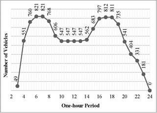
Demands for buses entering or leaving the system were determined based on the hourly variation of vehicle requirements over a typical weekday [19]. Figure 2 illustrates the estimated bus requirements for each of the one-hour periods considered. The fuel efficiencies of each bus type were set to 5.0, 9.5 and 15.0 km/gallon for ART, PAD and COM buses, respectively. Workshop yard capacities were established as 347, 338, 194, and 110 vehicles for WY1, WY2, WY3, and WY4, respectively.
We compare the four cases previously described with the present system situation, where each bus must return to its starting WY. The total daily fuel cost under the current circumstances was calculated by scheduling 1,092 daily jobs while imposing the latter condition. As said before, at present, the buses travel approximately 17,319 dead km/weekday, generating fuel costs of around 28 million COP$ per day (approximately 7,300 US$ per day).
3.2 Results for Case 1: original model run
In this case, we ran the original model with all constraints included. The total dead kilometers were 14,676.7, corresponding to a total daily fuel cost of 22,922.5 [COP $Thousands/day], which is 17.9% lower than the current system costs of 27,918.2 [COP $Thousands/day]. Table 2 shows the differences in dead km and the percentage difference by bus type.
Source: Based on [17].
Figure 2 Required operating buses per one-hour period (period 3 = 03:00 am, period 24 = 24:00 midnight)
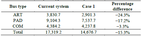
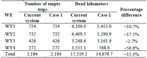
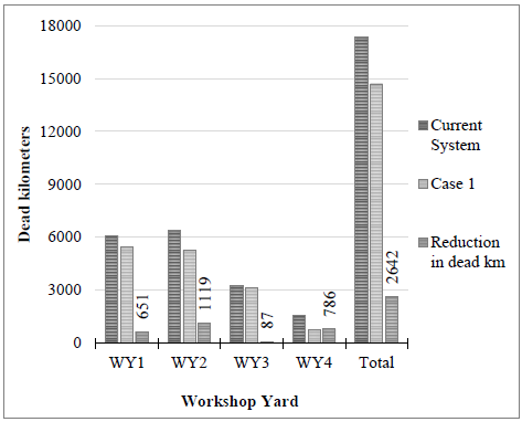
Table 4 Initial and final inventory of buses and capacity utilization by WY (Case 1).
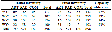
Source: The authors.
Table 3 depicts the total empty trips and dead km by WY. Additionally, Fig. 3 shows the dead km reduction for each WY. Regarding WY capacity utilization and observing the changes in inventory shown in Table 4, WY1 and WY3 have locations that favor the allocation of COM buses, while WY4 favors the allocation of ART vehicles.
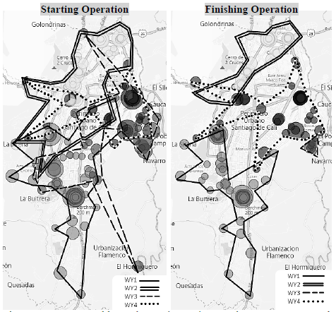
Fig. 4 shows the area covered by each WY when starting or finishing the operation. The size of each circle represents the number of jobs associated with each stop. Some allocations show long empty trips that can be further improved in the next cases.
3.3 Results for Case 2: relaxing licensees' participation constraints
In this case, we ran the original model relaxing the participation constraints (Eq. 8). The total dead kilometers were 13,989.3, corresponding to a total daily fuel cost of 22,070.1 [COP $Thousands/day], which is 21.0% lower than the current system costs. Table 5 shows the differences in dead km and the percentage difference by bus type. Details of dead kilometers and the number of empty trips by WY are shown in Table 6 and Figure 5. Note in Table 6 that although WY1 increases its associated dead km, the decreases in the other WYs generate a global reduction in this indicator.
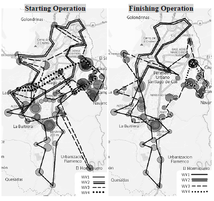
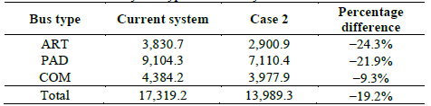
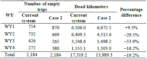
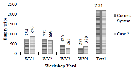
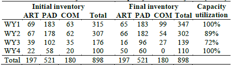
Table 7 Initial and final inventory of buses and capacity utilization by WY (Case2).
Source: The authors.
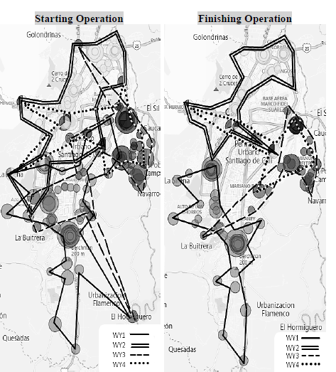
Table 7 shows the inventory changes from the start time to the finish time of the day and the capacity utilization of each WY.
Fig. 6 shows the area covered by each WY when starting or finishing the operation. Minor improvements with respect to the previous case (Fig. 4) can be observed. It is important to note that WY1 and WY2 cover the southern and northern zones of the city, respectively, while WY3 and WY4 serve the east and a few stops in the downtown of the city.
3.4 Results for Case 3: relaxing licensees' participation and WY capacity constraints
In this case, we ran the original model relaxing the participation constraints (Eq. 8) and modifying the capacity constraints (Eq. 6). By defining new decision variables ad_cap i , which represent the additional capacity that the model can suggest for each WY i, the constraints (Eq. 6) were redefined as:
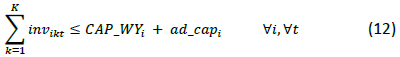
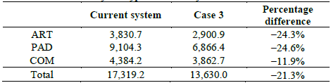
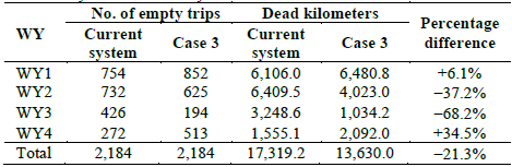
The total dead kilometers were 13,630.0, corresponding to a total daily fuel cost of 21,615.2 [COP $Thousands/day], which is 22.6% lower than the current system costs. Table 8 shows the differences in dead km and the percentage difference by bus type. Details of dead kilometers and the number of empty trips by WY are shown in Table 9 and Fig. 7. In this case 3, there are also reductions and increases in dead km for some WYs, but the total dead km are lower than those of the current system.
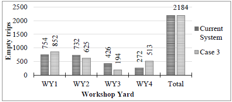
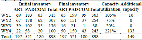
Table 10 shows the inventory changes from the start to finish time of the day, WY capacity utilization, and the additional WY capacity required to minimize fuel costs. WY4's additional capacity is key to minimizing the costs because it is near a stop that is one of the busiest. Also, WY3 would be using just 20% of its capacity, which suggests that it is not well located, or it is too close to Wy4.
Table 10 Initial and final inventory of buses, capacity utilization, and additional
Source: The authors.
Fig. 8 shows the area covered by each WY when starting or finishing the operation. Important improvements with respect to the previous case (Fig. 6) can be observed for the finishing operation. It is important to note that WY1 covers the south of the city, WY2 covers the north and west, and WY3 and WY4 mainly serve the east.
3.5 Results for Case 4: relaxing licensees' participation and WY capacity constraints and analyzing the operation over five consecutive weekdays
In this case, we ran the original model relaxing the participation constraints (Eq. 8) and keeping the capacity constraints as in Eq. 12, that is, allowing the model to generate additional Wy capacities. The rationale of this case is that the given initial inventory of buses at each WY may not be optimal. Therefore, this case also determines the optimal starting and finishing inventory of buses at each WY.
Source: The authors.
Figure 8 Area covered by each WY (Case 3). Note the more concentrated allocation of stops to each WY for the finishing operation.
Table 11 Summary of the main results of Case 4 by weekday with respect to the current system.
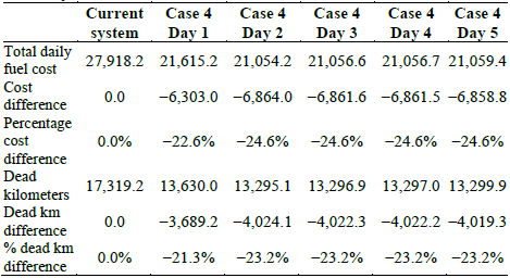
Source: The authors.
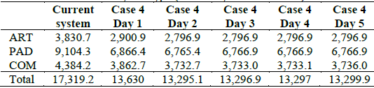
The results for day 1 are the same as those for Case 3. From this case, we keep the final inventories given in Table 10 as the initial inventories for day 2; then, we get the final inventories on day 2 as the initial inventories on day 3, and so on. From day 2, the empty trip distance stabilizes at approximately 13,300 dead km and the total daily fuel cost converges to a value close to 21,056 [COP $Thousands/day], which is 24.6% lower than the current system costs (Table 11). In addition, Table 12 shows the differences in dead km between case 4 and the current system, presented by bus type.
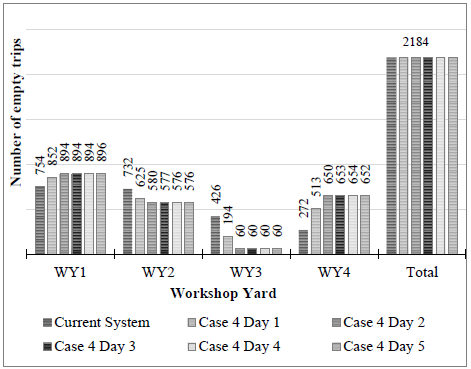
Fig. 9 shows that, for WY1 and WY4, the number of empty trips increases with respect to the current system. Conversely, for WY2 and WY3, they decrease. However, as illustrated above, the total dead km decrease. For all WYs, from day 2 to day 5, the number of empty trips converges. The small differences between consecutive days could be caused by integer rounding of the variables.
Fig. 10 depicts the reductions of dead km by WY with respect to the current system. Since WY1 and WY4 presented relatively small negative dead km reductions, then these workshop yards increased somewhat their associated dead km. On the contrary, WY2 and WY3 had positive dead km reductions between 2,000 and 3,000 dead km per day. Therefore, the total dead km reductions were meaningful. The numbers in Fig. 10 also illustrate the convergence of the applied method.
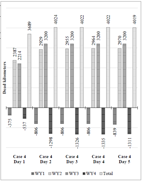
Table 13 illustrates the capacity utilization and the required additional capacity by WY at the end of each weekday. Note first that WY1 and WY4 are the two workshop yards that should increase their capacity.
Table 13 Capacity utilization (CU) and required additional capacity (AC) by WY over a five-weekday period (Case 4)._
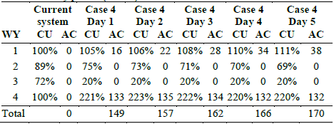
Source: The authors.
Conversely, WY3 uses a low percentage of its capacity. In the same way, Fig. 11 shows the inventory change by WY and type of vehicle over the five weekdays. The types of vehicles that should be allocated to each WY can also be identified in this figure. It is also important to note the convergence over time of the number of vehicles by type that should be allocated to each WY.
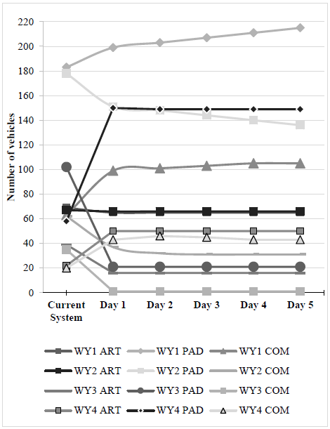
Source: The authors.
Figure 11 Final inventory of vehicles by WY and vehicle types over a five-weekday period (Case 4).
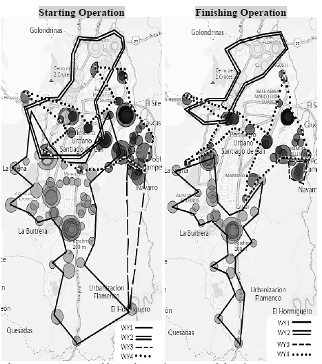
Fig. 12 shows the area covered by each WY when starting or finishing the operation on weekday 5. Relevant improvements with respect to the previous case (Fig. 8) can be observed for the WY3 starting operation. This can be explained by the low utilization capacity of this WY.
4 Conclusions
We presented an integer mathematical programming model to minimize the dead kilometers traveled by the vehicles of the mass transportation system in the city of Cali, Colombia. Four scenarios were analyzed and compared with the current transportation system. In all the scenarios, the vehicles were allowed to start and finish their jobs in different WYs. By gradually relaxing licensees' participation constraints, WY capacity constraints, and the initial inventory of buses in WYs, we obtained savings of total daily fuel costs ranging from 17.9% to 24.6%, corresponding to a range of yearly savings from 342,000 to 470,000 US$.
Additionally, the model identified those WY whose capacity should be increased. The results showed that there is one workshop yard (WY4) whose capacity should be increased by 123%. Also, another workshop yard (WY3) would use only 20% of its current capacity, suggesting its relocation or resizing. We could also find optimal initial vehicle inventories in WY at the beginning of a weekday, by iteratively running the model for five consecutive weekdays until obtaining convergence. By using stop location maps, we could generate visual areas of influence of each WY and observe their improvement by successive runs of the model.
Future works may include considering other costs, defining WY capacities depending on vehicle types, and simultaneously optimizing the WY locations.

