


 Inglés (pdf)
 Articulo en XML
 Referencias del artículo
 Enviar articulo por email
 Citado por SciELO
  Citado por Google
  Similares en
SciELO
Similares en
SciELO  Similares en Google
 Permalink
1. Introduction
Hydraulic pumps are one of civilizations earliest inventions and, taking into consideration its use in everyday life, they may be considered one of the most important. In 2000 BC, Egyptians created the shadoof to raise water, which is recognized by many historians as the first piece of turbomachinery. The Archimedean screw and the Chinese noria are other examples of early turbomachines. Since then, the development of new kinds and models of pumps have continuously evolved, concurrently with the scientific and technological knowledge of each era, ultimately having a big impact on the industrial development.
Today, it is difficult to imagine an environment, either industrial, commercial, or domestic, where the use of turbomachinery in general, or of pumps, in particular, are not relevant. Due to its extensive use, pumps represent an important part of the energy consumption in any country [1]. Therefore, identifying the best operating conditions for such equipment may significantly contribute to improve the efficiency of a fluid’s transport systems. The need for qualified personnel to efficiently design and operate pipeline systems is a challenge faced by the academy and the industry.
As a direct consequence of the relevance of the topic, turbomachines and pipeline systems are mandatory subjects at most mechanical engineering courses around the world. Traditionally, the students are trained to first calculate the energy losses, then to propose the system layout and sizing of the system according to the project demands¸ after that to select the proper pump and finally to determine the operating parameters under the specific condition. Most textbooks used in the applied fluid mechanics area [2-4] present this content using the simplest case: a single branch system operating under steady conditions. In fact, in most cases, undergraduate engineering courses tend to restrict their study to this case, for which a closed form analytic solution exists, even though its algebraic complexity requires an iterative solution.
Meanwhile, the industrial reality may be rather different and most of the real pipeline systems, such as gathering pipelines, transportation pipelines and distribution pipelines, may not be so easy to solve, as in many situations they must operate under transient condition.
Transient’s phenomena can be fast or slow as a function of, for instance, the variation of the pump operating parameters with time. Some examples of rapid transients are those that occur during the start-up and the shut-down of the pump [5], due to system valves' rapid operation [6], when the pump or its engine fails [7] and due to some hydrodynamic events associated with the pipeline systems operation [8]. In these cases, the transient is characterized by its very short duration and, generally, is not an intrinsic characteristic of the process. The effects of this transient are important from a technological point of view due to its incidence on the security and stability of the pump and pipe system. Thus, considerable research has been dedicated on this topic by means of analytical, numerical and experimental studies. Regarding to analytical modeling two assumptions are mainly used; the quasi-equilibrium condition [9,10] and the transient energy conservation equation [8,11].
On the other hand, the slow transient is an important process both from a technological and academic point of view, being frequent in the chemical, pharmaceutical, food, and mining processing industries. A typical example of slow transient is the fluid transfer between two reservoirs where the vertical height between the free surfaces varies with time. Then, it is possible to observe the similarity between this pumping system and the one taught in mechanical engineering undergraduate courses with the difference that in the last one there is no variation of the vertical distance between the fluid-free surface. Due to its origin, slow transients are unavoidable, hence the need for a better understanding of the phenomenon to effectively take advantage of it or to mitigate its consequences [12].
The bibliographical review carried out by the authors shows that little attention has been paid to study slow transient. Only two studies are reported in the technical or academic literature. In [13], the author presents a numerical solution to solve the slow transient that requires the use of several built-in math functions in Matlab to determine the flow rate a pump would deliver to a closed tank as a function of time. In [14] a novel analytical solution was obtained to describe the transfer of liquid between two open reservoirs with free surface heights varying with time. By using the model, it is possible to determine the fluid volume transferred from suction to discharge tanks.
Taking into consideration the similarity between the slow transient case above described and the steady flow pumping system that traditionally is taught in the mechanical engineering undergraduate courses around the world, the primary objective of the present work is to development an educational toolbox to solve the slow transient that take place in a single branch pumping system of a Newtonian fluids, with varying vertical levels between the suction and the discharge reservoirs. The theoretical study of the slow transient and the use of the toolbox allows the students a deeper insight about this transient in order to consolidate solid foundation in science and math, with expectation that students connect scientific and mathematical concept to engineering practice on this topic.
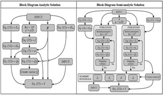
The educational toolbox is based on the mathematical model in the form of an ODE presented in [14], which was solved analytically for both the laminar and turbulent flow.
Through the toolbox’s inputs, students can study different practical applications related to the slow transients by setting different system layouts by means of suction and discharge piping system data, the fluid and its physical properties, and the pump by the head curve fitting coefficients. The outputs are shown in the form of graphs (volume transferred versus time and head versus flow rate) and tables.
2. Description of the hydraulic system under study
A simple, but pedagogically interesting, problem in water supply systems consists of a lower suction reservoir connected by a single pipeline system and a centrifugal pump to a higher discharge reservoir. This is the problem generally used to initiate the students in the study of pumps and pumping systems in most fluid mechanics texts, because of its simplicity. In practice, two situations may be distinguished: large and small reservoirs. Here, the word ‘large’ means that the water free surfaces stay at a constant level during the transfer. A more complicated problem arises in many industrial and technological applications when one or both reservoirs are small, i.e, surface levels vary during the transfer.
In both cases the pipeline system is often constituted by pipes of different materials with different absolute roughness in the suction and discharge sections, along with several different tube fittings and accessories. The diameter of the tubes may also be different in the suction and discharge section, as it is often the case, to help prevent cavitation.
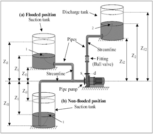
Fig. 1 shows the system just described. Here, Zi1 and Zi2, are the initial levels at the suction and discharge reservoirs and VR1 and VR2 are the velocities of their free surfaces. Hereafter, the suction and discharge lines are denoted by indices 1 and 2 respectively. The initial Zi1 and Zi2 values will vary until they reach their final values, Zf1 and Zf2, at the end of the operation. In this case, the flow rate, Q will also vary, and the time required to transfer a given volume of fluid is no longer given by the ratio between the transferred volume and the volumetric flow.
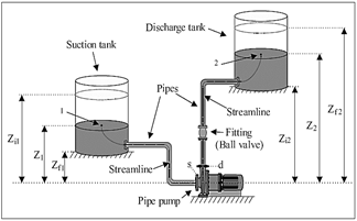
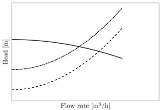
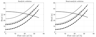
Fig. 2 shows the typical operating curves of such a pumping system. The pump curve is, obviously, unaltered whereas the pipeline system curve varies. The lower system curve in Fig. 2 shows the initial condition of the fluid transfer process, where the static head is small because the suction reservoir is at its higher level, and the discharge reservoir is at the lower level.
Source: Authors
Figure 2 Variation of the operating point in a system with varying fluid levels. (-) pump, (- - -) System’s initial manometric height, (- ( -) System´s final manometric height.
As time passes, the level difference increases, and the static head increases too. This shifts the system curve upwards, causes the operating point to go left, thus reducing the operation flow rate. The difference between the flow rate at the initial condition of the transient and the final one is called flow rate operational range.
3. Mathematical modelling of the problem
For the system in Fig. 1, the energy conservation Eq. for a streamline connecting points 1 and 2 at any given instant reads:
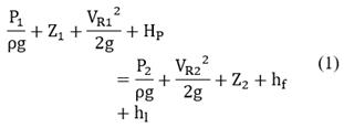
where distributed and minor energy losses are
Eq. (1) is only strictly valid for steady flows. Thus, our subsequent results are only valid when Z1 e Z2 vary slowly, i.e., when the free surfaces velocities VR1 and VR2 are small.
The distributed losses may be modeled by the Darcy-Weisbach equation and the minor losses may be modelled by K theory:
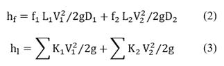
Where f1 and f2 are the friction factors of the tubes, L1 and L2 are the total tube lengths, D1 and D2 are their diameters and K1 and K2 are the loss coefficients. Finally, V1 and V2 are the fluid velocities in the tubes, not to be confused with the free surfaces’ velocities, VR1 and VR2.
If the whole system is now encircled by a control volume with moving boundaries at the free surfaces, the integral form of the mass conservation equation for an incompressible, stationary (for coherence) flow is VR1AR1 = VR2AR2 = Q, where ARi is the cross-sectional areas of the reservoirs, considered to be cylindrical, and Q is the volumetric flow rate. The mass conservation equation may also be written for any two sections of the tubing passing through the pump, yielding V1A1 = V2A2 = Q. Substituting those relations and eqs. (3-4) into Eq. (2) gives
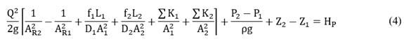
where
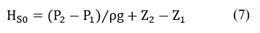
Regarding P1 and P2, two possibilities may be investigated. First, the reservoirs are closed, and the pressure varies due to the change in the free surface position, as it compresses or expands the gas above. Second, the pressures are constant as a process demand. In this case, a control system must be used to compensate the change in the free surfaces position, pumping gas in or out of the reservoir as the level falls or rises, respectively. The former situation was studied numerically [13] for smooth pipe systems. In their study, the author considers the variation of pressures but neglected the effect of the free surfaces’ velocities on Eq. (1). Our study focuses on constant pressures throughout the transfer. With this in mind, we rewrite Eq. (4) as
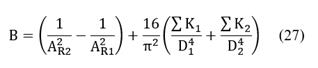
Where
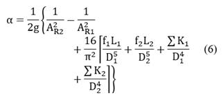
and
are constants. In Eqs. (6)-(7)
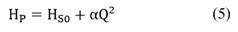
For centrifugal pumps, the head can be approximately modeled by
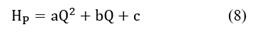
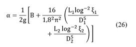
where a, b and c are experimental constants. Eq. (5) therefore becomes
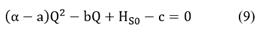
Applied initial and final conditions to Eq. (9) and solving for Q results in
where, from Eq. (7)
In the preceding analysis, all heights are input data except for Zf2. As the volume of fluid transferred out of reservoir 1 must go into reservoir 2, AR1 (Zi1 - Zf1) = AR2 (Zf2 - Zi2). But Q= - dυ1/dt, for dυ1 =AR1dZ1 and thus, Q= -AR1 dZ1 ⁄dt. Thus, integrating from t = 0 to t,
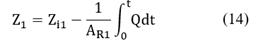
and similarly, for reservoir 2
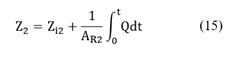
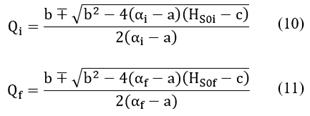
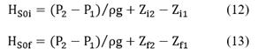
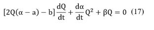
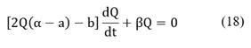
Combining eqs. (7), (12)-(15) and defining β = 1/AR2 + 1/AR1 results in HS0 = HS0i + β∫0 t Qdt. Substituting into Eq. (9) yields
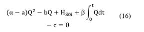
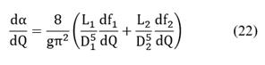
Differentiating in relation to Q and applying the chain rule, we finally obtain:
This equation is valid when reservoirs are not small enough to have large free surface levels velocities.
4. Analytic solution: constant values of f1 and f2
We initially consider f1, f2, K1 and K2 to be constants in Eq. (17). For f1 and f2 this is exact in the complete turbulence region of the Moody chart and is a good approximation in the rightmost part of the transition zone. The K coefficients of the minor losses are often considered constant in the literature. Thus, Eq. (17) yields
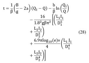
which is a separable and may be integrated between t = 0, when Q = Qi and t to give
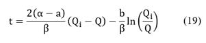
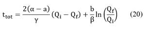
The total transfer time may be calculated by
5. Semi-analytic solution: time-dependent f1 and f2
Applying the chain rule to Eq. (18) results in:
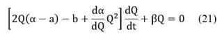
From Eq. (6)
From Haaland [15],
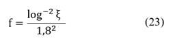
where
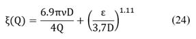
where
and
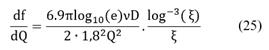
Where
Substituting Eqs. (22)-(27) into Eq. (21) and integrating:
where
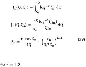
No closed form analytic solutions for integrals
6. Structure and development of the toolbox
The analytic and semi-analytic solutions obtained were implemented on an instructional toolbox. The MatLab® student version environment was chosen because of its wide use in the academic community. It also includes a tool for the development of interactive graphical interfaces (the Graphical User Interface Design Environment) allowing the user to develop a standalone application, i.e., it is not necessary to have the source code or Matlab® installed on one’s computer to run the program.
The basic philosophy for developing the toolbox is that it should be as simple as possible to create an integrated environment that makes it easy for students to use. This was done by combining existing mathematical functions with a routine developed by the authors.
The toolbox code is divided in five parts: inputs, code properties, equations, outputs, and user options. The input data, entered in SI units, can be divided into three categories:
Fluids and its physical properties: density and kinematic viscosity;
System parameters: length, diameter, absolute roughness and localized head loss coefficient of the suction and discharge sections; initial and final height of the suction reservoir’s free surface, initial height of the discharge reservoir free surface; pressure of the reservoirs free surfaces; geometric dimension of the reservoirs.
Pump parameters: the coefficients of the pump’s performance curve. Alternatively, the user can insert the values of flow rate and head for the pump selected using the 'DETERMINE COEFFICIENTS' button and the code then uses the Matlab® ‘polyfit’ function to obtain the fit coefficients. Fig. 3 shows the layout of the toolbox.
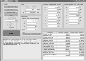
The outputs are presented in three schemes:
A table, containing time-dependent information, such as Re (the Reynolds number), f and Q at the beginning and at the end of the transfer, and global information, as the total volume transferred and
A field for notifications, indicating the progress of the calculation and notifying eventual problems, as shown in the left-bottom part in Fig. 3.
Graphics showing the characteristic curves at the beginning and the end of the transfer, and other showing Q = Q(t), as presented and discussed in the Section 7 of this work.
Before closing, the code prompts the user to save the semi-analytical results to an extension .xlsx file, if desired. Finally, the toolbox offers the possibility to save, load and clean the inputs, to plot the graphs together or separately, in addition to having a help button, which describes in detail how to use the toolbox. Fig. 4 illustrates the operation of the code.
7. Results and analysis
To demonstrate the capabilities of the toolbox developed, three study cases were created representing important industrial applications of academic interest: the influence of the fluid nature, the selection of the pump, and the effect of the suction reservoir position. All these topics are addressed in our Fluid Machinery courses, under steady conditions. Thus, the transient approach presented opens a path to allow the student a broader and more realistic vision of the matter. Input data for the study cases are listed in Tables 1-3. The first column in Tables 1-3 represents the combination of inputs for the different study cases.
Table 1 Toolbox inputs for suction and discharge tanks.
|
|
|
|
|
|
|
|---|---|---|---|---|---|
| 1 | 19.63 | 38.48 | 12 | 6 | 15 |
| 2 | 78.54 | 176.70 | 15 | 3 | 15 |
| 3 | 50.26 | 78.53 | 7.5 | 2.5 | 12 |
| 4 | 50.26 | 78.53 | -2.5 | -7.5 | 12 |
Source: Authors
Table 2 Toolbox inputs for suction and discharge pipeline.
|
|
|
|
|
|
|
|
|
|
|---|---|---|---|---|---|---|---|---|
| 1 | 3 | 90 | 0.1 | 0,075 | 2 | 15 | 3 | 2.25 |
| 2 | 5 | 200 | 0.15 | 0.10 | 5 | 20.5 | 0.15 | 0.10 |
| 3 | 7 | 50 | 0.075 | 0.050 | 7.5 | 12.0 | 0.015 | 0.010 |
Source: Authors
Table 3 Toolbox inputs for the pump.
|
|
|
|
|
|
|---|---|---|---|---|
| 1 | -160000 | 0 | 45 | 40 |
| 2 | -14256 | 0 | 24 | 40 |
| 3 | -19440 | 0 | 36 | 120 |
| 4 | -3888 | 0 | 21 | 180 |
| 5 | -111465 | 0 | 35 | 30 |
Source: Authors
Table 4 Summary of the results for the SC1
| Water | Slurry | |||||
| Analyt | Semi-analytic | Error (%) | Analyt | Semi-analytic | Error (%) | |
|
|
1E08 | 1.33E05 | 1E08 | 3.14E04 | ||
|
|
1E08 | 1.80E05 | 1E08 | 4.14E04 | ||
|
|
1E08 | 1.18E05 | 1E08 | 2.80E04 | ||
|
|
1E08 | 1.60E05 | 1E08 | 3.70E04 | ||
|
|
0.0573 | 0.0575 | 0.4 | 0.0573 | 0.0583 | 1.7 |
|
|
0.0573 | 0.0576 | 0.5 | 0.0573 | 0.0584 | 1.8 |
|
|
0.0573 | 0.0575 | 0.4 | 0.0573 | 0.0580 | 1.2 |
|
|
0.0573 | 0.0575 | 0.4 | 0.0573 | 0.0581 | 1.4 |
|
|
37.755 | 37.72 | 0.1 | 37.755 | 37.64 | 0.3 |
|
|
33.435 | 33.40 | 0.1 | 33.435 | 33.20 | 0.7 |
|
|
198.53 | 198.68 | 198.53 | 199.17 | ||
Source: Authors
7.1. Study case 1 (SC1): Influence of the fluid nature
An important criterion for selecting turbomachinery is the type of fluid to be transferred, but due to the impossibility of anticipating the working fluid, manufacturers characterize pumps by using water.
Here we assess the behavior of a pumping system for water and for a slurry. In this case, the slurry is formed by a mixture of water and tantalum (( = 940 kg/m3 and ( = 4.25E-06 m2/s), a very common Newtonian fluid in the mining industry. In both cases, the suction pump is in a flooded position. The characteristic curve of the pump used is defined for water and thus viscosity corrections are required. The system and the pump characteristics are defined in line 1 of Tables 1-3. Table 4 shows the main results obtained in SC1 with both the analytic and semi-analytic solutions.
For the analytical solution, the value of f is the same for both fluids, because it only depends on the duct relative roughness. For the semi-analytic solution, the values of f and of Re varies, as seen in Table 4. The maximum difference between these solutions was below 2% at the end of the transfer. Such small differences were expected, once the flow regime is in the complete turbulence region of the Moody chart for both fluids.
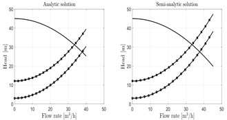
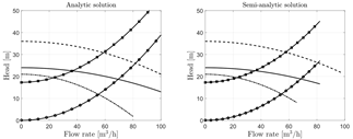
The system transient behavior is shown by means of the characteristic curves as shown in Fig. 5, for the semi-analytic and the analytic solutions. No difference between the curves for both fluids are seen, even though the difference in physical properties is significant. This is due to the fact that the flow is in the complete turbulence region and, therefore, f depends only on the relative roughness.
Source: Authors
Figure 5 Graphical output. Influence of the fluids viscosity: (-) pump, (- - -) System´s initial manometric height for water, (- ( - () System’s initial manometric height for slurry (- o -), System´s final manometric height for water (- ( o), System's final manometric height for slurry.
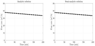
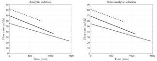
The flow rate operational range, i.e. the difference between Qi and Qf during the transient, is 4.32 m3/h antttotd is 198.5 minutes for both fluids. The transient flow rate is shown in Fig. 6 for both fluids and solutions. It can be seen that in any case the transfer time is the same and, therefore, the four curves overlap regardless of the fluid viscosity and method of solution.
As discussed in the Fluid Machinery course, when centrifugal pumps are used with highly viscous fluids, it is necessary to make performance corrections. The operating parameters obtained with a pump characterized for water, should be corrected using correction factors for flow rate, head and efficiency. One of the most used tables for these corrections was proposed by the Hydraulic Institute (USA). After the corrections, it is possible to verify that, when compared with water, the flow rate and head decrease and the shaft power increases, resulting in a smaller pump efficiency. The viscosity corrections are widely used in the oil-gas and in the chemical industries, amongst many others.
In SC1, the students are expected to practice technical skills such as designing and sizing a pipeline system with all tube fittings and accessories necessary, selecting a high viscosity fluid for an industrial application, verifying the different existing methods to carry out the viscosity correction and, finally, analyzing the results.
Finally, it is worth noting that, as normally discussed in class, depending on the application and the demand, volumetric pumps are usually recommended for high viscosity fluids rather than radial pumps.
7.2. Study case 2 (SC2): Influence of the selected pump
The proper selection of a pump for a particular application, whether in a steady or in a transient process, is extremely important. It determines the efficiency in the fluid transport and, consequently, the associated costs. Additionally, this guarantees that the system and the pump operate as reliably and efficiently as possible.
In this sense, this analysis will discuss how to apply and extend the pump selection criteria studied in the standard courses for systems in transient applications. For this purpose, three situations will be discussed here: two well and one intentionally not well selected pump. The criterion adopted was that the pump must operate in the preferred operating region (POR), i.e. with 0,7QBEP ≤ Qop ≤QBEP. This is rather important for transient processes where the operating point change continuously during the operation.
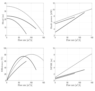
For all cases, the same small-size pumping system is considered for water transfer between two reservoirs. The system and the pump characteristics are defined in line 2 of Tables 1-2 and for pumps in line 2-4 of Table 3 (hereafter designated P1, P2 and P3). Fig. 7 shows the performance curves for the three pumps.
As shown in Table 5, the difference in f varies from 6.2 to 13.9% in the suction line and from 4.4 to 10.0% in the discharge line, with the lowest value for P2 and the highest for P3. Here the flow regime is in the transition zone. In both cases, the lowest error occurs at the beginning of the transient and the highest at the end. This difference is reflected in the characteristic curves shown in Fig. 8 where the semi-analytic curves are slightly different for the initial and final times but the analytical curves are not.
Table 5 Summary of the results for the study case 2.
| P1 | P2 | P3 | |||||||
| Analyt | Semi-analyt | Diff. (%) | Analyt | Semi-analyt | Diff. (%) | Analytic | Semi-analytic | Error (%) | |
|
|
1E08 | 1.6E05 | 1E08 | 1.9E05 | 1E08 | 1.66E05 | |||
|
|
1E08 | 2.5E05 | 1E08 | 2.9E05 | 1E08 | 2.50E05 | |||
|
|
1E08 | 8.70E0 | 1E08 | 1.4E05 | 1E08 | 6.97E04 | |||
|
|
1E08 | 1.3E05 | 1E08 | 2.1E05 | 1E08 | 1.04E05 | |||
|
|
0.0197 | 0.0212 | 7.07 | 0.0197 | 0.0210 | 6.19 | 0.0197 | 0.0212 | 7.07 |
|
|
0.0197 | 0.0223 | 11.65 | 0.0197 | 0.0214 | 7.97 | 0.0197 | 0.0229 | 13.90 |
|
|
0.0197 | 0.0207 | 4.83 | 0.0197 | 0.0206 | 4.36 | 0.0197 | 0.0207 | 4.83 |
|
|
0.0197 | 0.0215 | 8.37 | 0.0197 | 0.0209 | 5.74 | 0.0197 | 0.0219 | 10.04 |
|
|
69.36 | 68.49 | 1.31 | 81.73 | 80.89 | 1.04 | 54.57 | 55.21 | 1.52 |
|
|
36.56 | 35.01 | 2.32 | 58.86 | 58.03 | 1.41 | 29.58 | 28.61 | 3.27 |
|
|
1057.1 | 1075.7 | 804.5 | 814.2 | 1126.58 | 1151.76 | |||
Source: Authors
Source: Authors
Figure 8 H-Q system and pumps curves: (-)P1, (---) P2, (- ( - () P3, (-o-) System's initial manometric height, (-( -) System´s final manometric height.
Next, the influence of the selected pump on the system's operating parameters will be analyzed. As observed in Table 5 and Fig. (8-left), for P1 Qi = 69.14 m3/h, Qf = 36.06 m3/h, and the operational range is ΔQ = 33.08 m3/h. For P2, these values are Qi = 80.88 m3/h, Qf = 58.02 m3/h and ΔQ = 22.86 m3/h and for P3, Qi = 69.72 m3/h, Qf = 28.61 m3/h and ΔQ = 41.11 m3/h. It can also be observed in Fig. (8-left) that because of the transient, the static head term in the system curves increases from zero, at the beginning of the transient, to 17.3 m at the end of the process. This corresponds to the vertical distance between the free surfaces in the suction and discharge tanks, at the end of the transient.
From these results, students have all the necessary information to make an efficiency and energy consumption analysis. According to the premises and objectives of SC2, in the first and second analyses, pumps were selected with the condition that the best efficiency point (BEP) is around the maximum operating flow rate at the beginning of the transient operation.
Pumps are designed to operate at the BEP, with an acceptable range defined by the POR criterion. From the efficiency curves in Fig. 7(bottom left), we note that in the first analysis P1, the pump efficiency varies from 75.6 % for Qi to 58.5 % for Qf. The BEP for this pump coincides with the maximum flow rate,
Similarly, in the second analysis, the efficiency is 78.5% for Qi and 66.9 % for Qf. The BEP for this pump occurs at 100 m3/h (81.1%). The POR criterion is met when the pump flow rate is 70 m3/h and the efficiency is 72.9%.and thus the pump operates in the POR during 43,0 % of the time. For the final analysis, the efficiency for Qi is 53.83 %, and for Qf is 26.0%, the BEP is at 160 m3/h where the efficiency is 83.9%. The POR criterion is met when the pump operates at 112 m3/h with efficiency around 73%. Since Qi is less than
The shaft power required by the pump in a particular application is another important parameter for selecting the most appropriate pump. For P1, the average shaft power consumption during the fluid transport is 5.3 kW, which represents 104.3 kWh of energy consumed during the operation. Similar calculations for P2 and P3 result in 9.24 kW (125.8 kWh) and 6.8 kW (127.9 kWh) respectively.
From these results, we note that for a given volume to be transferred, P3 operates with the lowest efficiency, consumes more energy, spend more time, and always operates out of the POR. It consumes 1.1 % more energy and spends 29.3 % time than P2 and consumes 18.5 % more energy and spend 6.6 % more time than P1.
These results point out to the need for a correct selection of the pump to guarantee the efficient transport of fluids.
After SC2, the students should have a better understanding of the technical criteria for the selection of a pump by assessing the interdependence between the operating parameters. Another important goal of this study is associated with the improvement of the student's skill for searching information about pump manufacturers and performance curves for different pump models through contact with pump manufacturers and traders.
7.3. Study case 3 (SC3): Influence of the system configuration
Here students will evaluate the influence of the suction tank's position on the selected pump performance and the possibility of cavitation, an important aspect in the pump’s operation, especially when pumping fluids at high temperatures.
The system and the pump characteristics are defined in lines 3 and 4 of Table 1, line 3 of Table 2 and line 5 of Table 3. The analysis will consider the same system and pump and two different suction tank positions: flooded suction pump, where the liquid is held at a level above the suction port of the pump, and non-flooded suction pump, where the opposite occurs, as shown in Fig. 10. In both analyses, the fluid is water at 70°C (( = 978 kg/m3 and ( = 0.41E-06 m2/s).
Source: Authors
Figure 10 (a) Suction tank above the centreline of the pump (flooded) (b) suction tank under the pump (non-flooded).
The toolbox automatically identifies the suction tank position because pumps operating in non-flooded condition have negative initial and final heights (it considers the centerline of the pump as the reference). The transferred volume was also kept constant for both analyses. The results obtained are shown in Table 6.
In this case, when a pump operates flooded, the static head is smaller than when the pump operates non-flooded. As the transferred volume in both cases is the same, at the end of the transient, both system curves are shifted upward by the same amount, as shown in Fig. 11(left and right). The calculations show that
Source: Authors
Figure 11 Characteristic curves and flow rate for systems with different positions of the suction tank (-) pump, (- - -) System´s initial manometric height for nonflooded suction, (- ( - () System´s final manometric height for nonflooded suction, (- o -) System´s initial manometric height for flooded suction (- ( o), System´s final manometric height for flooded suction.
The shaft power of the pump used in SC3 may be fitted by the model N = 1.9 + 0.0556Q, the efficiency by η = 3.967Q - 0.0771Q2 and the NPSH, by NPSH = 0.5457 + 0.0543Q+0.0017Q2 with N in kW, in %, NPSH in m and Q in m3/h. Considering these equations and Table 6, we verify that, for the semi-analytic solution, Qi = 28.84 m3/h Qf = 24.66 m3/h, indicating that the pump operates between 50.3 % and 51.0% efficiency. For the non-flooded suction configuration, Qi = 23.04 m3/h, Qf = 17.75 m3/h operating between 50.5% and 46.1% efficiency. In these cases, the BEP occurs at 26 m3/h (51 %) and the pump operates during all the time in the POR.
To avoid cavitation, it is necessary that NPSHa ≥ NPSHr + SM, where the value of the security margin, SM, is often specified in-house by design consultants, but pump manufacturers will always offer advice. Typically, SM=1.5 m is enough.
The NPSHa can be calculated by NPSHa = (Patm - Pv) ⁄ ρg ± ∆Zs - (Σhf + Σhl)s, where ∆Zs is the vertical distance between the free surface of the suction tank and the suction port of the pump. This term is positive if the suction of the pump is flooded and negative otherwise. The last term on the RHS represents the energy losses in the suction pipeline.
As the flow is transient, cavitation is analyzed for the worse possible condition i.e. at the end of the transient, when the head reaches its lowest (positive) value for the flooded configuration and the head its greater (negative) for non-flooded configuration.
Table 6. Main results for flooded suction pump and non-flooded suction pump.
| Flooded suction | Non-flooded suction | |||||
|---|---|---|---|---|---|---|
| Analyt. | Num.l | Error (%) | Analyt | Num. | Error (%) | |
| Re1i | 1E08 | 3.31E05 | 1E08 | 2.71E05 | ||
| Re1f | 1E08 | 4.97E05 | 1E08 | 4.07E05 | ||
| Re2i | 1E08 | 2.83E05 | 1E08 | 2.10E05 | ||
| Re2f | 1E08 | 4.25E05 | 1E08 | 3.15E05 | ||
| f1i | 0.0138 | 0.0159 | 13.20 | 0.0138 | 0.0163 | 15.33 |
| f1f | 0.0138 | 0.0162 | 14.81 | 0.0138 | 0.0168 | 17.85 |
| f2i | 0.0138 | 0.0159 | 13.20 | 0.0138 | 0.0156 | 11.53 |
| f2f | 0.0138 | 0.0162 | 14.81 | 0.0138 | 0.0160 | 13.75 |
|
|
28.84 | 28.22 | 2.15 | 23.64 | 23.05 | 2.53 |
|
|
24.66 | 24.05 | 2.47 | 18.31 | 17.75 | 2.90 |
| Ttot (min) | 563.63 | 576.84 | 718.67 | 739.22 | ||
Source: Authors
For the flooded configuration, the NPSHa = 8.76 m and NPSHr + margin = 4.32 m, showing that the pump will not cavitate. However, the non-flooded configuration will cavitate, because NPSHa = 0.77 m and NPSHr + margin = 3.54 m. In the last case, the toolbox warns the students to take corrective measures.
In SC3, the targets of the students are designing and sizing a pumping system, to analyze the possibilities of cavitation according to setting the pumping system up and, to define corrective actions when cavitation occurs. Results show that cavitation is more likely to occur when the suction pump is flooded. When the fluid temperature is high (>45°), it is strongly suggested that the flooded suction pump condition should be first analyzed and, if possible, implemented.
8. Conclusions
This work deals with an important application in mechanical engineering, consisting of the pumping of a Newtonian fluid on a simple branch hydraulic system in which the vertical distance between the suction and discharge reservoir varies. In this case, the flow rate and many other characteristics quantities of the process, as the Reynolds number and the friction factor, are time dependent. Knowledge from several areas of mechanical engineering were used to obtain the solution proposed: differential equations, fluid mechanics, programming, numerical methods, and turbomachinery.
Solutions previously obtained by authors were implemented in a simple, friendly and intuitive toolbox using the MatLab package, that allows students to configure different pumping systems in order to obtain the main pump operating parameters and assess the operating conditions for the system and the pump in transient conditions. Although not illustrated in this paper, the toolbox developed can simulate a system with pumps associated in series or in parallel, by providing the curves corresponding to the pumps’ association is used. The same applies to Newtonian fluids other than water, provided again that the corrected pump curve is used. The only present limitation of the toolbox is tackling with laminar flow. This capability was not included because it is seldom encountered in the engineering practice. Nevertheless, creating and implementing such a module presents no challenge.
To illustrate the toolbox’s operation, three study cases connected to academic interests were discussed. The first assessed the influence of fluid properties, showing the importance of viscosity corrections when the used pump is characterized for water. However, it should be noticed that viscosity corrections were only indicated but not carried out. The second allows the students to assess the importance of the appropriate pump selection. Applying the efficiency criteria, it was demonstrated that pumps should operate most of the time in the preferred operating region for better economic management of the pumping systems. The third is associated with the influence of the suction tank position. Depending on the fluid temperature, on the suction line characteristics and on the pump selected, the simulation showed that cavitation may occur, and corrective measures should be taken.
Finally, we believe that the toolbox developed can provide students of undergraduate mechanical engineering courses with a practical tool for studying and understanding time dependent pumping systems.

