2.1. Modified model Sal'nikov for chemical energy supplied to a muscle sarcomere

From a macroscopic scale, a striated muscle is formed by muscle fibers composed of myofibrils. Zooming a single myofibril reveals that each consists of cylindrical units called sarcomeres [¹⁵]. Sarcomeres are the largest ordered multi-protein assemblies; their most remarkable components are thick and thin filaments interlaced, nearly identical in length [¹⁶]. The thin filament comprises actin, troponin, tropomyosin, and myosin II motors from the thick filament at this microscopic scale. Each myosin molecule has two cross bridges that attach cyclically to the actin filament and move the actin along the myosin filament. As both filaments overlap, the sarcomere length gradually decreases. The visible result of summing the contribution of all sarcomeres will be the development of macroscopic force and muscle shortening [¹⁷,¹⁸]. The hydrolysis of ATP provides the energy required to complete the attaching-detaching cycle to ADP and Pi occurring at the myosin catalytic domain. The chemical reaction is coupled to a mechanical response [¹⁹].

Sal'nikov's modified model does not pretend to describe sarcomere at these scales. Instead, it focuses on the biochemical aspect of energetics requirement to make muscle contraction possible. In this sense, a sarcomere is comparable to a chemical reactor where a reaction occurs through ATP supply (macro-sarcomere), and the supply rate constrains the reaction time course. In fact, at the molecular level, the myosin cross-bridge is the transducer that interconverts chemical energy (derived from ATP) to mechanical work [²⁰]. Thus, the proposed model intends to understand how thermal gradients can couple to biochemical oscillations of energetic species relevant to muscle function, i.e., ATP, rather than explain details of the sarcomere mechanism.

Sal'nikov’s modified model proposed before [²] was based upon three differential equations (eq. 1-3), including two chemical (Y and Z) species and heat conduction. A parameter γ controls transition from pure thermal instabilities (γ = 0 ) to mixed thermal-chemical instabilities (γ = 0 ).

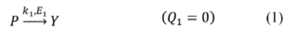
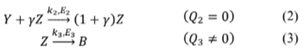
In this case, thermal dependence is linked to the conversion Z^k3 →B (the exothermic reaction with enthalpy Q₃ ≠ 0 ), where k3 takes the form of eq. (4):

and ∇T = 1/T_a - 1/T Table 1 summarizes the parameter values used to simulate system dynamics according to eq. (1)-(4). In the set of governing differential equations, V is the reactor volume, Cp, the heat capacity of the mixture, S is the reactor surface area, χ is the surface heat transfer coefficient and Ta, the surrounding temperature. The concentration of each chemical specie is presented in lower caps. Heat loss is modeled as a simple Newtonian heat transfer, assuming a well-stirred solution.:

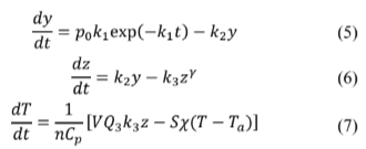
To couple several of Sal'nikov’s modified systems, the actual model is discretized using the finite differences method. Then eq. (5)-(7) will look like an equation set defined by eq. (8)-(10), keeping in mind that the value for γ is set to γ=1 along the paper. When rewritten, the differential equations are set, and the term p ₀ k ₁ exp(-k ₁ t) was assumed constant under chemical pool approximation for P specie and denoted v _p . Denoting by i the spatial step associated with a discrete compartment and by super index j a time step, then:

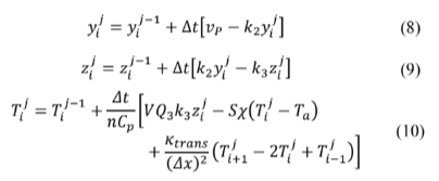
Here, k _trans represents the heat transfer coefficient between two adjacent compartments. Note that coupling was made only in Fourier's heat transfer law, and there is no chemical exchange. Doing k _trans = 0, in eq. (10), reduces it to eq. (7). It makes sense when thinking about the selectivity of a cell membrane.

2.2. Configuration entropy tool to characterize the system

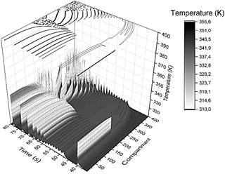
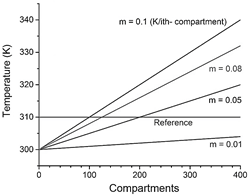
As mentioned, the present study aims to model chemical energy supply over time to a macro sarcomere unit. After bringing together enough sarcomeres, a myofibril is confirmed. As a result, the chemical energy input of myofibrils is a series of eq. (8)-(10) takes place. A sample of 400 compartments was arranged in a 1-dimensional linear array, and the initial thermal gradient (slope of the linear gradient, m), thermal pulse applying-time (t _app ) as well as pulse amplitude (T_Δ) were varied to construct a phase diagram (see variables tested in Table 2). The compartment's initial temperature T_i, where i-th is defined according to the equation of a straight line T _i = m i + T _max where T _max = 300 k and the slope m varies between 0.01 and 0.1 K/i-th compartments (Fig. 2). Pulses were applied each 5 s, starting from 40 s to 70 s and affected only the first half of the compartments ( i = 0 to i = 200). A typical 2D contour plot, like that in Figure 1, is drawn when running simulations with the combinations of variables previously described and summarized in Table 2. (Fig. 1 shows the evolution of the 1-dimensional array on the "Compartment" axis projected in the temporal axis and the "Temperature" axis).

Source: Own elaboration.

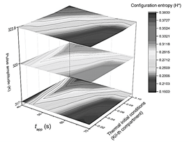
Figure 1 3D profile showing the system's time evolution when a thermal pulse of amplitude 323.9 K was applied at t _app = 40s, and the slope of the initial linear gradient was 0.1 K/i-th compartment. At the top of the box is sketched the corresponding 2D contour plot, which will be the starting point for configuration entropy analysis. The X-axis corresponds to the i-th compartment (from compartment i = 0 to i = 400), the y-axis corresponds to the time, and the z-axis is the temperature (the gray color scale facilitates the interpretation of the contour plot). 

Source: Own elaboration.

Figure 2 Thermal initial conditions imposed at time zero to each compartment, defined by the value of the slope m of a straight line. Reference temperature (green horizontal line, 310 K) is determined as the minimum temperature reached by the system in the frame of interest (40 - 80 s). 

Naturally, covering different initial thermal conditions and applying thermal pulses of different intensities or at other times will be reflected in an extensive collection of plots. Each 2D natural contour plot is resized to obtain helpful information from those pictures until receiving sides of the same length L. Thus, raw images are reduced to 5000 × 5000 pixels and displayed in black and white mode, associating each black pixel with one and a white pixel with a 0. This way, the same image is interpreted as a matrix filled with zeroes or ones. All this pre-processing stage prepares a particular image to be analyzed through configuration entropy as described by Andraud et al. [²¹,²²]. The 2D contour plots generated from each simulation by employing configuration entropy are treated as disordered morphologies and characterized with a descriptor that describes their fractal structure [²³]. This method has been used to describe fractal landscapes to clay soil samples and even fat, connective tissue [²³-²⁵]. This analysis method qualitatively describes the 1-dimensional array response to different conditions. It provides information about the system's behavior only under the restrictions imposed. An analytical stability analysis from eq could achieve a more general analysis. (8)-(10).

The prepared image is analyzed through a sliding square cell of side l. For a particular position of the cell, the number of pixels with value one contained in the cell is counted. Once the whole image is examined, it is computed N_k(l), the number of cells containing k active pixels, and N(l), the total number of visited cells. The probability associated with the state of the cell is thus defined as p _k (l) = N _k (l)/N(l) and the corresponding entropy is:

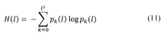
which measures the uncertainty associated with the set of possible states the cell of size l may attain. H(l) is an effective descriptor of the likelihood of the random pixel distribution which may occur inside a cell of size l. It is noteworthy that l cannot approach the size of the lattice since p _k (l) would lose any real meaning, thus the condition l < L/4 is fixed. To examine the image structure at different length scales, the cell size is progressively increased. In accordance with those increments, entropy H(l) changes, being necessary normalize its value in order to compare entropy values corresponding to different cell sizes. Then, for each l value the normalized entropy H*(l) = H(l)/H _max(l) is computed, where H _max (l) = log (l ² + 1). H*(l) is called the configuration entropy of 2-dimensional morphology of the image [²¹-²³]. Fig. 3 presents the configuration entropy analysis obtained from successive 2D contour plots where slope of the initial thermal gradient is 0.1 K/i-th compartment and pulse amplitude is T _Δ =323.9k. Value for configuration entropy allows distinguishing clearly when pulse is applied at t _app = 40s (Fig. 4a, H* = 0.4095) and t _app = 70s (Fig. 4b, H* = 0.2746). Qualitatively, the resulting image with more black pixels is associated with a higher H* number (Fig. 4a has more black pixels than Fig. 4b). Fig. 5 summarizes the configuration entropy values obtained in the space of the parameters presented in Table 2.

Source: Own elaboration.

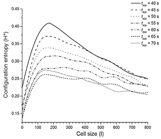
Figure 3 Configuration entropy was obtained after applying thermal pulses at different times. Configuration entropy (H*) vs. analysis block size (l) of a 2D contour plot when T_Δ is fixed to 323.9 K and the slope of the initial linear gradient is 0.1 K/i-th compartments. H* value is calculated from the maximum of each curve. 

Source: Own elaboration.

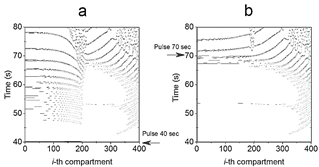
Figure 4 2D thermal contour plot generated after the Pulse perturbed the system at (a) 40s (H* = 0.4095) and (b) 70s (H* = 0.2746), respectively. 

Detailed configuration entropy values are reported in Fig. 7 and 8 when pulse amplitude was fixed to 317 (Fig. 7) and 323.9 K (Fig. 8). Again, the highest bars are contained in the region described above. This zone qualitatively implies a disordered morphological 2D structure associated with ordered structures. As the emergence of black pixels is tied to the number of oscillations exhibited in time, the zone with the highest entropy of Fig. 5 exhibits more oscillations (see 2D plot in Fig. 4a, where the pulse was applied for 40 s and has a higher H*₄₀ =0.4095) than other regions (2D plot in Fig. 4b, where the pulse was applied at 70 s, with lower H*₇₀ = 0.2746).

Source: Own elaboration.

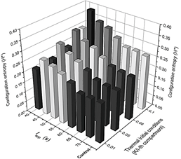
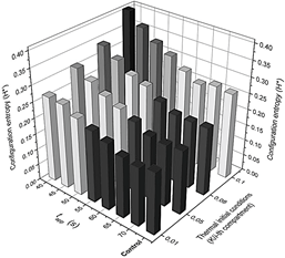
Figure 5 Summary of the results obtained using the configuration entropy analysis for different pulse amplitudes. Phase diagram collection summarizing the system's response after being thermally stimulated. Each plane corresponds to a different pulse amplitude response while varying on each of them the pulse-applying time t _app , and the slope m of initial thermal conditions (x-axis and y-axis). 

3.1. Overall effect of a thermal pulse

In these conditions, oscillatory chemical specie Z could be identified as ATP in a real fiber when restoring chemical energy is prioritized. Set of eq. (8)-(10) provides a compartmentalized energy supply model under such stressful conditions. A characteristic course time of temperature developed in a single 1-dimensional array is presented in Fig. 6. Fig. 8(d-f) presents the oscillatory transient in Z specie, which naturally is coupled to the thermal profile.

Source: Own elaboration.

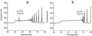
Figure 6 Time course of the first compartment's temperature for the plane at T_Δ= 317k related to (a) high and (b) low configuration entropy zones. In (a) pulse is applied at 45 s, and in (b) pulse is applied at 70 s. The slope of the linear gradient was 0.1 K/i-th compartment and 0.01 K/i-th compartment, respectively. 

Source: Own elaboration.

Figure 7 Detailed configuration entropy values reached by the system after being stimulated thermally by a pulse of 317 K. 

Source: Own elaboration.

Figure 8 Detailed configuration entropy values reached by the system after being stimulated thermally by a pulse of 323.9 K. Pulse applying time and the slope of the thermal linear gradient were varied successively according to values reported in Table 2. Figures 6 and 7 are a 3D representation of the same 2D phase diagram presented in Fig. 3a. 

At this point, asking for the other compartments that complete the ideal muscle fiber outlook becomes logical. Each of them could be characterized with a plot of temperature vs. time or chemical concentration vs. time. However, the image obtained from the 3D plot of the fiber's time history is processed by the constitutive entropy method (a typical 2D contour plot shown in Fig. 1) instead of providing the evolutionary information of the system separately in this way. As a result, each image is numbered from 0 to 1. The advantage of the configuration entropy tool lies in the possibility of discriminating with quantitative criteria an extensive collection of plots. This information is summarized in three 2D phase diagram plots generated after the maximum peak amplitude was set to 317, 320, and 323.9 K (Fig. 5). It can be seen that the zone, with the highest entropy value, is restricted to pulse applying time ranging from t_app = 40 s to 45 s. In the other coordinate, it is contained between m = 0.08 and m = 0.1k/i-compartment.

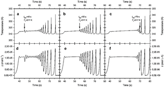
In quantitative terms, if the thermal Pulse is applied before inherent oscillations start, the system responds with an oscillatory train (this is the case of Fig. 9(a-b)). The number of changes is proportional to the configuration entropy value in the time-compartments space, as shown in Fig. 3-4. However, if perturbation has no effect at the time of application of the Pulse, its amplitude is not comparable with the system's maximum amplitude. Correspondingly, the vibration of Fig. 9c applied at t _app = 70 s falls in a valley, making its relative amplitude not identical with the adjacent thermal spikes. Therefore, it does not significantly change the shape of the single-compartment temperature histories and the 2D contour plots are almost unchanged (see Fig. 7-8. Pulse and control applied at 70 s, i.e., Unperturbed systems exhibit similar entropy values). Therefore, it does not significantly change the shape of the single-compartment temperature histories, and the 2D contour plots are almost unchanged (see Figs. 7-8. Pulse and control applied at 70 s, i.e., Unperturbed systems exhibit similar entropy values). Instead, changes disappear once the Pulse is applied (figure not shown).

Source: Own elaboration.

Figure 9 2D graphs providing an overview of a single compartment (i = 1 ) response after being stimulated thermally. Each graph corresponds to a different thermal (a-c) or chemical (d-f) response. The slope of the initial thermal gradient was 0.1 K/i-th compartment, and pulses of T_∆ = 317 K were applied at times t_app = 45, 55, and 70 s. 

Besides the aspects concerning the pulse amplitude and when the system is perturbed, initial thermal conditions tend to increase configuration entropy. Linear thermal gradient slope, m, notoriously affects the behavior of the final half of the fiber, and even in the absence of perturbation, thermal spikes appear. A comparison between 2D contour plots from Fig. 4a and Fig. 4b hints that the upper part of both plots is the same, independent of the Pulse. In this sense, initial thermal conditions are absorbed like a thermal pulse. According to Fig. 2, at time t=0, the last compartment should start with a temperature between 320 - 340 K if m is picked from m = 0.05 to m = 0.1 K/i-th chamber. However, when m = 00.1 K/i-th compartment, the last room is not heated until the reference value of 310 K. Precisely, for the latter, Figs. 7-8 reports the minimum configuration entropy values concerning other possible initial conditions.

3.2. Discussion

When a muscle fiber is exhausted after high exercise loads, depletion of ATP is expected near the Ca²⁺-ATPases [²⁶]. Oxidative metabolism or pools of energetically representative chemical species like PCr cannot maintain a continuous ATP feed at high rates and will be exhausted sooner or later. This ATP is essential to keep the Ca²⁺ ions exchange, which plays a fundamental role in the attaching-detaching cycle of myosin-actin filaments. At first sight, an ATP deficit at this level implies stopping all the machinery related to muscle movement. Nevertheless, being quiet is not as bad since an additional chemical impulse could lead to irreversible damage to the tissue [²⁷]. The inconvenience would not be the ceasing of machinery's activity. Still, the time it takes to recover could be reduced if ATP is restored, and not precisely by the oxidative metabolism pathway.

These ideas were developed in a previous paper [²], where a chemical energy inlet was modeled for a single sarcomere. In such cases, it showed the relevance of chemical oscillations coupled with the local thermal gradient in stressing conditions to replenish levels of a chemical specie of interest, i.e., ATP. The set of equations proposed was based on a modified Sal'nikov model and summarized in the eq. (1)-(3). Through numerical analysis, parameters presented in Table 1 were found to reproduce chemical oscillatory behavior in the presence of thermal instabilities, i.e., doing γ = 1. This condition was the starting point for the present work since the main goal was to evaluate a thermal gradient synergistic effect. Either in the form of a heat pulse, as proposed by [⁴], or a thermal gradient arising from intense muscular work alongside a muscle fiber, non-isothermal conditions modify system dynamics. They could be an emergency mechanism to overwhelm muscle fatigue locally.

Under energetic stressing conditions [¹,²⁸], myocytes from rat exhibit glycolytic and sustained ATP oscillations. If, as proposed in the set of eq. (1)-(3), These oscillations are gradually introduced in γ in autocatalysis along an oscillating thermal gradient. A chemical and thermal explosion is observed when the γ = 1 state is reached. It is the portrait of a single reactor unit.

Thus, a single reactor is an oversimplified system hosting some reactions inside a sarcomere with enough detail to capture the relation between the chemical species that promote oscillatory behaviors. A coupling of several identical reactors, connected through heat exchange only, will lead to the idea of a myofibril chemical energy supplier. In other words, the model of eq. (8)-(10) fuels each i-th sarcomere with an inlet of chemical specie Z, associated with ATP. This scenario requires the definition of a finite volume for the reactor to connect several units that resemble a macro myofibril. Still, this parameter is kept constant since the interest is centered on the reactions.

Additionally, the 1-dimensional array of reactors (ideal myofibril) is sensitive to thermal changes. Experimentally, the effect of thermal dependence on muscle function is studied with localized thermal stimulus over muscle tissue or single cells (c.f. [⁷,²⁹,³⁰]) rather than using single myofibrils. This limitation centers the discussion on the qualitative results shown here rather than a numerical comparison against available data.

The way the compartmentalized model distributes chemical energy when no thermal pulse or initial thermal gradient is present is precisely a near identical repetition of the Z profile and thermal profile from the first cell i = 1 to i=400. This ideal case does not show an appreciable change between cells in time despite including thermal exchange from each compartment I with their surrounds. However, when initial thermal conditions of the compartments are forced to behave linearly, following the equation of a straight line, different slopes m reveal a notorious change, especially near the last portion of the compartments. This difference when changing initial thermal conditions is a consequence of Fourier's heat transfer coupling because this law forces two adjacent rooms to exchange heat at the fastest rate possible [⁵], and being this process slower or more evident between compartments with different temperatures i = 0 and i = 400.

The system is more perturbed with the highest value for m (see Fig. 2). In effect, Fig. 4a shows that, even when a thermal pulse is applied, if m=0.1 K/i-compartment, the last compartments respond with thermal spikes and, conversely, chemical spikes in Z (Fig. 9(a-d)). In general, phase diagrams from Fig. 5 confirm that this value of m is obtained as the highest value for configuration entropy. Even a system unperturbed by a heat pulse has a minimum configuration entropy associated if a thermal profile is imposed since the beginning. Alternatively, in other words, chemical and thermal oscillations arise only as a consequence of the linear initial thermal conditions for each compartment. For this reason, the height of the bars for the undisturbed (control) system in Fig. 7-8 is comparable with bars obtained after a pulse is applied for 70 s (where the Pulse has no visible effect).

Nevertheless, suppose a homogenous thermal gradient would be sufficient to activate all the compartments, i.e., to increase the amount of Z with the thermal burst. In that case, it is more likely that a natural fiber is under a non-homogenous thermal gradient. The linear gradient proposed here is only an ideal case, illustrating how the compartments 'feel' the thermal burst at different times. First compartments are the first affected by thermal explosions, and to the extent we move away to the last boxes, shots are delayed. For this reason, the time course of temperature corresponding to the first compartments seems to be shifted in time concerning the last rooms. Besides, it implies that the chemical supplier model oscillates in time, but the temperature and, conversely, the concentration of Z, varies among compartments at a given time.

In addition to an initial thermal linear gradient, the system is perturbed with a heat pulse, and the observed response varies in function of Pulse applying time and pulse amplitude. Pulse affected only half of the cells, i.e., two hundred compartments. Pulse applying time is a critical parameter if the pulse amplitude is not higher than the maximum amplitude of the oscillation when it is applied. Therefore, between 40 s and 60 s, a pulse starting at 317 K has a significant impact in terms of configuration entropy because, in this range, the amplitude of the Pulse is greater than the temperature of the system (~315 K) (see Fig. 9(a-b)), promoting an oscillatory behavior just as the Pulse is applied. Something similar occurs with initial thermal conditions since for m=0.5 to m=0.1 K/i-compartment, the initial temperature is over the reference temperature of the system, 310 K (see Fig. 2).

Contrary to non-homogenous initial thermal conditions, a thermal pulse impacts homogenous thermal initial conditions similarly. That means synchronizing the fiber's chemical energy production simultaneously and among thermally stimulated compartments. This thermal synchronization has been recognized as a valuable tool, for example, to pace embryonic hearts [⁷].