


 Inglés (pdf)
 Articulo en XML
 Referencias del artículo
 Enviar articulo por email
 Citado por SciELO
  Citado por Google
  Similares en
SciELO
Similares en
SciELO  Similares en Google
 Permalink
1. Introduction
Turbulent flow is a state of fluid motion, which could be found in industrial applications and in the natural environment. Heat exchangers, chemical reactors and burners are industrial devices where turbulent flow can be found, whereas in the atmosphere, rivers and oceans could be found natural turbulent flows. 1. A large number of fluid flow applications in the industry are turbulent since turbulence itself enhances mass and heat transfer 2.
Turbulence modeling is mainly addressed from three main approaches, Direct Numerical Simulation (DNS), Large Eddy Simulation (LES) and Reynolds-Average Navier-Stokers (RANS) 3. DNS is out of reach for engineering applications; only small domains with moderate Reynolds numbers have been successfully simulated under this approach 4-6. RANS models are less computationally expensive, but small-eddies scales are not solved. LES is a trade-off between DNS and RANS models in terms of accuracy and computational cost. Simulations of industrial applications under the LES approach had been restricted by the high computational cost of such models 2. Nevertheless, the access to High-Performance Computing (HPC) hardware with the right meshing approach could allow to power experimental studies with LES for industrial combustion applications 7.
Despite successful modeling of several turbulent flow configurations using RANS models, some challenges remain. The reliability of those turbulence models have been questioned for applications where unsteady boundary layer separation and vortex shedding are of great importance 8. Flows over bluff bodies are commonly found in industrial devices for burning gas, liquid and pulverized solid fuels. Unfortunately, the proper representation of turbulent flow quantities on the bluff body zone will rely on the capability of the model for capturing unsteady boundary layer separation and vortex shedding phenomena 9,10.
Safavi and Amani 11 have conducted an assessment of RANS, LES, and hybrid turbulence models for non-premixed swirl-stabilized flames, where RANS models do not entirely capture the unsteady boundary layer separation close to the bluff body zone. As result, an underestimation of the primary recirculation zones, a slower mixing rate on the bottom of the flame, and some unphysical behaviours of the flame were found. De Santis et al. have conducted an investigation where several LES sub-grid models were tested for diffusion swirling flames. It seems that jet penetration into the highly rotational flow field, formed by the swirl air supply, is still very hard to accurately quantify by the LES sub-grid models assessed 12. Despite the remaining challenges, both authors highlight the great importance of the instantaneous velocity field resolution accomplished by the LES model.
From a practical point of view, LES could deliver useful results during the early development stages of combustion devices. However, a suitable instantaneous velocity field resolution seems to be a key point in the accuracy of the results obtained and the computational cost for carrying out the simulations. Therefore, the present work aims to assess the influence of the instantaneous velocity field resolution on the reliability of simulation results for a common combustion flow configuration.
2. Background
2.1. Main governing equations
Continuity (eq. (1)) and conservation of momentum (eq. (2) governs flow of fluids.
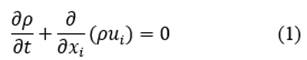
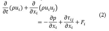
In combustion process, density (ρ) is a variable that depends on pressure, temperature and species concentration. In eq. (1-2), u denotes a three-dimensional velocity vector, the sub index i and j take values from one to three denoting the three Cartesian direction (x,y,z) and F i represents body forces. The τ magnitude in eq. (2) denotes shear stress tensor.
Since mass transfer plays an important role in combustion phenomena should be presented as a governing equation for species concentration, which takes the form of eq. (3).
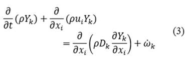
Y represents the species mass fraction, ω reaction rate of each species, D species mass diffusivity and sub-index 𝑘 each analyzed speciess. In combustion applications, temperature depend on the thermodynamic and chemical state at each time and location. As combustion takes place, chemical energy is released as thermal energy and resulting enthalpy is obtained by simultaneously solving an energy transport equation. However, if a single mass diffusion coefficient is used, the Lewis number is in the order of unity. It can be expressed energy equation as eq. (4) shows.
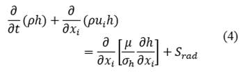
The contribution of heat transfer by radiation is taken into account by the source term (S rad ). Such contribution is computed by solving the Radiative Transfer Equation (RTE) known as P1 model, further information about this model could be found in the work published by Cheng 13 an later included by the work of Siegel and Howell 14.
2.2 LES turbulence modeling
The smooth parallel fluid motion characterizes laminar flow, where each streamline remains almost undisturbed. Nevertheless, at high enough Reynolds number the vorticity turns fluid motion chaotic 6. Large eddies extract energy from the mean flow, meanwhile small eddies dissipate energy into heat due to molecular viscosity. Large eddies are the most energy-containing and highly conditioned by the geometrical boundaries 15. These important findings led to an alternative approach for dealing with turbulence, where turbulence quantities of the large motion structures are directly computed, while the near isotropic part is modeled with the sub-grid models. LES turbulence modelling approach began with the work of pioneer as Smagorinsky 16, Lilly 17 and Deardorff 18.
2.2.1 Sub-grid-Scale models
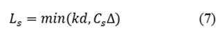
The modeling of sub-grid-scales stress tensor have led to the development of several models for such purpose, Wall-Adapting Local Eddy-Viscosity (WALE) 19, Algebraic Wall-Modeled LES (WMLES) 20 and Dynamic Kinetic Energy Subgrid-Scale models 21. However, for the scope of the present work the Smagorinsky-Lilly 16 and Dynamic Smagorinsky-Lilly models 22,23 will be used and therefore analyzed in more details. For the Smagorinsky-Lilly model, the turbulent viscosity is computed by eq. (5)-(7).
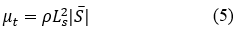
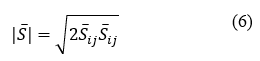
 is the mean strain rate tensor and L
s
is the mixing length under sub-grid scale, which considers Von Kármán constant (k = 0.41), wall closest distance (d), cutoff width (∆) and Smagorinsky constant (C
s
). Lilly obtained C
s
= 0.23, considering an isotropic turbulence in the inertial subrange of boundary layer. However, these constant values result in a damping overestimation of the large scales fluctuations near solid boundaries 24,25. There is a general agreement that values around 0.1 for the Smagorinsky constant provides the best results for a wide range of flows.
is the mean strain rate tensor and L
s
is the mixing length under sub-grid scale, which considers Von Kármán constant (k = 0.41), wall closest distance (d), cutoff width (∆) and Smagorinsky constant (C
s
). Lilly obtained C
s
= 0.23, considering an isotropic turbulence in the inertial subrange of boundary layer. However, these constant values result in a damping overestimation of the large scales fluctuations near solid boundaries 24,25. There is a general agreement that values around 0.1 for the Smagorinsky constant provides the best results for a wide range of flows.
Germano et al. 22 and Lilly 23 developed a procedure for estimating Smagorinsky constant, mainly based on the resolved scales of fluid motion in a dynamic manner. A new filter  (cutoff width) is applied and the resulting information from the two-filtering operation is used for the constant computation, further information could be found in Germano and Lilly work 22,23.
2.3. Mesh resolution index
According to Pope criteria 8, at least 80 % of the turbulent kinetic energy contained in instantaneous velocity-field should be resolved and the other 20 % may be modelled by an eddy-viscosity sub-grid model. Eq. (8) shows a metric used for assessing the resolved percentage of turbulent kinetic energy.
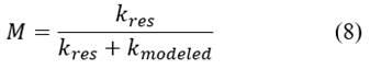
M takes values from zero to one, preferred values should be more than 0.8, which correspond to more than 80% of the turbulent kinetic energy resolution. Eq. (9)-(10) show how to compute the part of turbulent kinetic energy resolved (k res ) and the part modeled by the Sub-Grid Scale (SGS) model 𝑘 𝑚𝑜𝑑𝑒𝑙𝑒𝑑 .
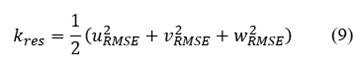
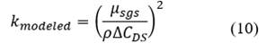
RMSE indicates the Root Mean Square Error of velocity components, μ sgs is the sub-grid turbulent viscosity, C DS is the sub-grid dynamic constant and ∆ is the turbulence resolution length scale or the cutoff value. However, as the mesh aspect ratio departures from unity the assumption made for the estimation of the resolution length scale become less accurate 8,11.
3. Experimental and numerical setup
The Sydney non-premixed swirling SM1-flame 26, from the Clean Combustion Research Group at the University of Sydney, it is used as benchmark in the present work. This flame shows two important features, a swirling air supply and circular bluff body, both features commonly found in combustion engineering devices.
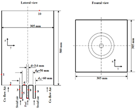
The SM1 methane flame was experimentally studied by means of a swirl burner, which is coaxially located in an air co-flow. The co-flow is conformed of a rectangular wind tunnel of 305 mm for the transversal section. The swirl burner is made of a fuel nozzle of 3.6 mm, coaxially located at a circular bluff-body of 50 mm of diameter. The bluff-body is located inside an annular section, which will be used for supplying the swirling air to the flame. Fig. 1 shows a scheme of the computational domain used for simulations of the SMA1 flame. The domain is a rectangular box with 500 mm of length, with a square transversal section of 305 mm, where a fuel nozzle of 3.6 mm is coaxially located.
Source: The authors.
Figure 1 Lateral view and frontal view of the computational domain used for the simulation of the SMA1 flame.
The flow field variable measured were axial velocity and tangential velocity components, being estimated the velocity magnitudes for the exit plane at fuel nozzle (axial velocity Uj = 32.7 m/s), annular swirl-primary air supply (axial annular-velocity Us = 32.7 m/s and tangential annular-velocity Ws = 19.1 m/s) and co-flow of secondary air supply (axial velocity Ue = 20 m/s). Additionally, species concentration and temperature profiles were sampled for SMA1-flame. Further information about the experiments for this flame, calibration and uncertainties of the measurements made by means of those techniques could be found in 27-29.
An annular and coaxial section of 5 mm of width surrounds the fuel nozzle. The domain shown on Fig. 1 is meshed, resulting in a mesh conformed by 3 794 825 hexahedral elements. The mesh is finer close to the bluff body, with a minimum element size in the axial direction of 0.1 mm. The rectangular zone, which has 0.5 m of length, was meshed using two blocks. The first block has a length in the axial direction of 300 mm. This is the block connected to the bluff body, which was meshed with a minimum element size in the axial direction of 0.1 mm and a maximum of 0.5 mm. The second block is 200 mm of length, which was meshed with a minimum element size in the axial direction of 0.5 mm and a maximum of 1 mm. Fig. (2) shows two views of the meshed domain for the SMA1 flame.

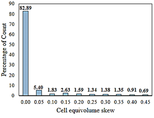
Fig. 3-4 show the histograms of Cell equivolume skew and the orthogonal quality of the SMA1-flame mesh. Two mesh quality criteria were used, the cell equivolume skew and the orthogonal quality. About 82 % of the mesh cells count have a cell equivolume skew between 0 and 0.08. The other cells percentage have at least a cell equivolume skew less than 0.69. According to Ajit and Fergal, values of cell equivolume skew of 0 to 0.25 are considered excellent, 0.25 to 0.5 are good and 0.5 to 0.75 are fair 30. About 95 % of the mesh assessed is excellent and the other 5 % still being good.
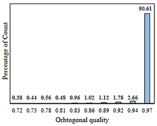
Considering the orthogonal quality metric, more than 93 % of the mesh has an orthogonal quality close to unity, which means that the mesh is almost orthogonal, values typically obtained from an O-grid meshes. According to Santana et al. 31, such orthogonal quality values suggest that the mesh is very good.
The simulations were conducted using the professional software ANSYS-Fluent, which implements the FVM for solving the governing equations. Two types of simulations were conducted in this flame case. First, an incompressible steady state simulation using the SST 𝑘−𝜔 turbulence model, which was used for the initialization of the LES simulation (three dimensions and transient simulation).
In this case, the Eddy-Dissipation model with single global reaction was used for accounting for chemistry-turbulence interaction. For the RANS precursor simulation (incompressible steady state simulation using the SST k - ω turbulence model) were solved momentum, turbulent kinetic energy, turbulent dissipation rate, energy, species mass fraction and P1 RTE equations by means of the FVM. The Pseudo-Transient Coupled algorithm was used as a pressure-velocity algorithm. First-order-upwind numerical scheme was used for turbulent kinetic energy and turbulent dissipation rate equation terms. Second-order-upwind numerical scheme was used for the discretization process of momentum, energy, species mass fraction and P1 RTE equation terms, including pressure gradient terms. It was established as convergence criteria residual for energy and radiation in the order of 1 × 10⁻⁹ and for the rest of the residual in the order of 1 × 10⁻⁶. The results from the precursor simulation were used for initializing the LES simulation, which is a fully 3D transient simulation. A LES turbulence modeling approach was adopted, using the Dynamic Smagorinsky-Lilly sub-grid model. A Bounded Second Order Implicit Transient Formulation was used for the time discretization terms. Also, Bounded Central Differencing numerical scheme was used for the discretisation of momentum equation terms, considering the mesh spacing used a time step in the order of 1 × 10⁻⁶ s. The convergence criteria was established by means of a residual in the order of 1 × 10⁻⁶ for the energy and P1 RTE equations and for the rest of the residual in the order of 1 × 10⁻³.
3.1. Boundary conditions
Fig. (1) shows the computational domain for the SMA1-flame, the different boundaries are highlighted with red dots. Table 1 summarises the boundary conditions for the SMA1-flame, where essentially three BC types are found. For the precursor simulation, turbulence intensity was estimated by the empirical model proposed by Andersson et al. 2. Nevertheless, for the LES simulation, a more realistic boundary condition should be provided. Fluctuations of velocity components and turbulent kinetics energy should be provided at the velocity-inlet boundary condition. In order to accomplish such initial conditions Vortex Method is used with a simplified linear kinematic model for computing streamwise velocity fluctuations 32,33.
Table 1 Boundary conditions for the SMA1-flame. aBoundary conditions ID are reflected on Fig. 1. bNo slip condition are applied to all walls.
| BC-IDa | Type | Axial Velocity (m / s) | Tangential Velocity (m / s) | Temperature (K) | Heat flux (W / m 2 ) |
|---|---|---|---|---|---|
| 1 | wall | - | - | - | 0 |
| 2 | velocity-inlet | 20 | - | 300 | - |
| 3 | wall | - | - | - | 0 |
| 4 | swirl-velocity-inlet | 38.2 | 19.1 | 300 | - |
| 5 | wall | - | - | - | 0 |
| 6 | wall | - | - | - | 0 |
| 7 | velocity-inlet | 32.7 | - | 300 | - |
| 8 | wall | - | - | - | 0 |
| 9 | wall | - | - | - | 0 |
| 10 | outflow | - | - | - | - |
Source: The authors.
Additionally, for the BC-ID 2 and 4 molar fractions of XO2 = 0.21 are established. For the BC-ID 2 molar fraction of XCH4 = 1 is established.
4. Results and discussion
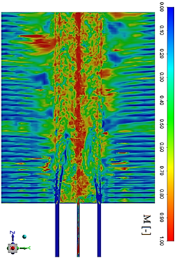
Fig. 5 shows the contour of the quality index M, whereas M approaches unity, the closer to a DNS will be the resolution of the turbulent kinetic energy contained in the instantaneous velocity field. It can be appreciated that the zone with the best resolution of turbulent kinetic energy is located at the central zone of the combustor. The zone of the swirl-air-inlet, close to the bluff body and downstream is quite unresolved.
Source: The authors.
Figure 5 Contour of quality index M for assessing the resolved percentage of turbulent kinetic energy with respect to the total turbulent kinetic energy.
However, according to Pope 34 M is highly dependent of ∆ value and at the same time the computation of ∆ becomes less accurate where mesh aspect ratio is far from unity. As can be appreciated from Fig. 2, the mesh aspect ratio is far from unity almost everywhere, only in the zone close to the fuel nozzle and the combustor center-line this parameter is close to the unity.
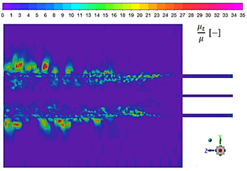
Another approach to quantify the resolved turbulent kinetic energy is the viscosity ratio, which is directly related to the Large Eddy Simulation Index Quality (LES_IQ) proposed by Celik et al. 35. Values of viscosity ratio below 20 suggest that more than 80 % of turbulent kinetic energy is resolved. Fig. 6 shows the contour of viscosity ratio, where can be corroborated the failure of index quality M on the zones with a height mesh aspect ratio for assessing the resolved turbulent kinetic energy. Nevertheless, from the figure can be appreciated that still insufficiently resolved the turbulent kinetic energy. Several spots on the shear layer zone showed a resolution smaller than 80 %.
Source: The authors.
Figure 6 Contour of sub-grid viscosity ratio for assessing the resolved percentage of turbulent kinetic energy with respect to the total turbulent kinetic energy.
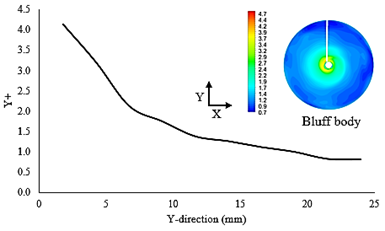
On the other hand, zones where near wall resolution become important like close to the bluff body wall, Y + parameter is highly important to quantifying the sub-layers physics.
Unfortunately, the meshing process is not a straightforward process and no clear consensus appears in the literature about how to build a heigh quality LES-Mesh. Nevertheless, some common ground has been reached in relation to near-walls resolution and the Y + parameter. According to Launchbury this parameter has to be less than one and should be always checked for the walls of interest 3. Fig. 7 shows the Y + distribution over the bluff body wall, where seems that only above 19 mm in the radial direction of the bluff body the Y + is less than one. The figure indicates that near-wall resolution over this important wall for the present case study is insufficient.
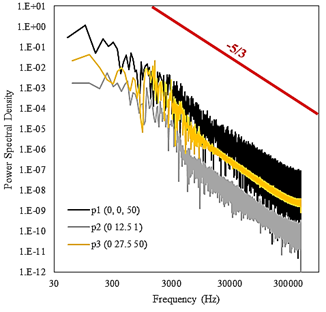
Turbulent flow is a transient phenomenon, but at some time a statistically stationary state is reached. Such state is not reached until the turbulence is fully developed. In order to find out when the flow is fully turbulent, a spectral analysis is required. According to Lacaze et al. when the turbulent flow is fully development the Power Spectral Density (PSD) show a decay rate of about -5/3 36. For the PSD analysis three points were sampled, when simulation reached 50000 time-steps a Fast Fourier Transform was computed from the axial velocity time series measured. Fig. 8 shows the location of the sampled points and the PSD of the axial velocity at those points.
As Fig. 8 shown the −5 3 Kolmogorov law is accomplished, suggesting that is reached the fully turbulent state after 50000 time-steps and a proper time resolution by using a time-steps of 1 x 10⁻⁶ s. Then, flow field statistics was restarted, computing time-averaging and mean quantities over 30000 time-steps more.
4.1. Flow field data analysis
SMA1-flame flow field is characterized by two main recirculation zones and a neck region. The first recirculation zone is induced by the flow separation behind the bluff body wall, commonly called base recirculation zone (BRZ). This recirculation zone enhances the upstream mixing process, making this zone acting as a perfect stirred reactor and providing a constant ignition source for the flame. The second recirculation zone is aerodynamically induced, a swirl-air-inlet induces further downstream a vortex breakdown bubble (VBB), which stabilizes the flame close to the flame-limit where local flame stingiest can appear 37. The BRZ has a toroidal shape and reaches the stagnation point at z = 43 mm from the bluff body wall. The VBB is observed during experimentation at combustion center-line, downstream from z = 76 mm to z = 96 mm. The neck region is formed about z = 55 mm downstream and extend in radial direction about half of bluff body diameter 38.
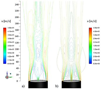
Fig. 9 shows the contour lines of the time-averaged axial-velocity for the LES and mean axial velocity for the RANS simulation. Both turbulence modeling approaches manage to capture the neck, the BRZ and the VBB zone. Nevertheless, both models differ regarding the neck location with respect experimental observations. The neck location for the LES simulation is further located in about 15 mm downstream than experiment observations. RANS simulation shown that neck is further located about 5 mm downstream than experiment observations. LES agrees with the experiments regarding the location of the BRZ and the VBB zone. The precursor simulation reaches the stagnation point for the BRZ and VBB zone closer to the bluff body wall than experimental data and the LES simulation.
Source: The authors.
Figure 9 Contour lines of time-averaged instantaneous-axial-velocity and mean axial-velocity, a) LES with sub-grid Dynamic Smagorinsky-Lilly and b) RANS precursor with SST k-ω models.
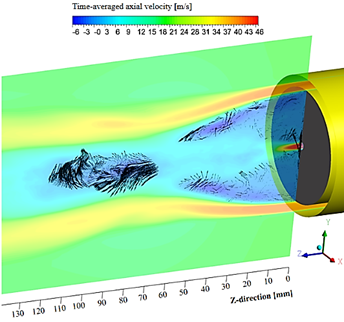
Fig. 10 shows the contour of time-averaged instantaneous-axial-velocity with an imposed vector plot over the BRZ and VBB zones for the LES model. The figure shows a strong velocity decreasing of the fuel jet along the combustor center-line until reaches the stagnation point at the VBB zone.
Source: The authors
Figure 10 Time-averaged axial velocity contour and vectors plot over BRZ and VBB area.
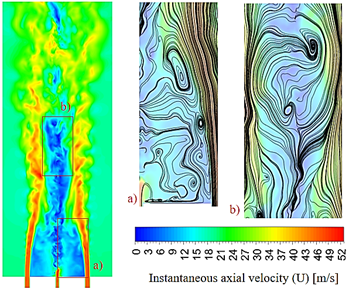
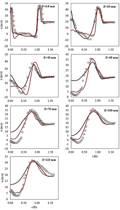
Vectors plot shows the highly rotational flow motion of fluid parcels at the BRZ and VBB zones. Fig. 11 shows the contours of instantaneous axial-velocity with a zoomed in of streamlines for the BRZ and VBB zone. It can be realized by the formation of a high-velocity shear-layer surrounding the combustor center-line and the two main recirculation zones. The flow separation behind the bluff the body and the vortex breakdown at downstream of combustion center-line stretch the high velocity shear layer forming the neck. The insufficient resolution of the instantaneous velocity field in the shear layer region, seen on Fig. 6 could contributes to the difficulty of the LES model to properly locate the neck. Fig. 13 shows the profiles of time-averaged axial velocity for the LES simulation, mean axial velocity profiles for experimental measurements and precursor simulation. It turns out that LES and RANS simulation fairly capture the main velocity-profile shape.
Source: The authors.
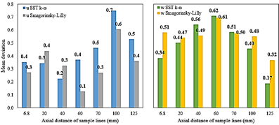
Figure 12 Mean deviation of time-averaged axial and tangential velocity for LES simulation and mean deviation of mean axial and tangential velocity for the RANS (u is referred to axial velocity and w is referred to tangential velocity components).
Source: The authors.
Figure 13 Profiles of experimental measurements of mean-axial velocity (squares), LES time-averaged axial-velocity (red line) and precursor simulation mean axial-velocity (black line).
Fig. 12 shows the mean deviation of time-averaged axial and tangential velocity for LES simulation, as well as mean deviation of mean axial and tangential velocity for the RANS simulation. Five radial profiles showed a lower mean deviation of axial velocity for the LES than axial velocity for the RANS simulation. At z = 20 mm and z = 40 mm the mean deviation of axial velocity was lower for the RANS simulation than axial velocity for the LES simulation. In the case of the tangential velocity, LES shown a lower deviation than RANS simulation in only two radial samples, at z = 40 mm and z = 60 mm. At the other radial samples, the RANS simulation outperforms the LES simulation.
4.2. Species and temperature data analysis
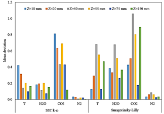
Fig. 14 shows the mean deviation of temperature and species mass fraction for the LES and RANS simulations. As the figure shows the results from the precursor simulation globally outperforms the results from LES simulation. However, from a qualitative point of view the RANS simulation shows some unphysical behavior, like the presence of a flame temperature peak behind the bluff body wall.
Source: The authors.
Figure 14 Mean deviation of time-averaged temperature for LES simulation, mean temperature for RANS simulation, mean mass fraction of H 2 O, CO 2 and N 2 for LES and RANS simulation.
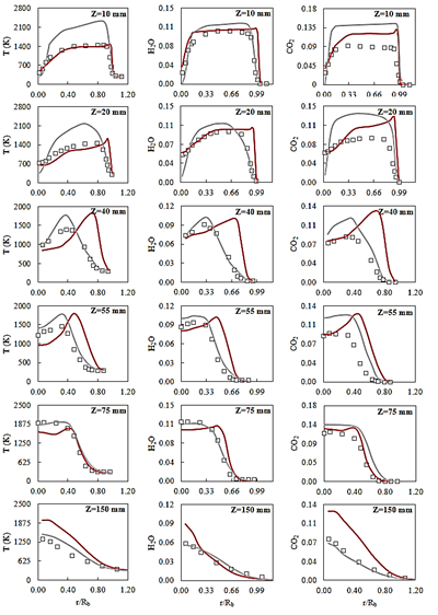
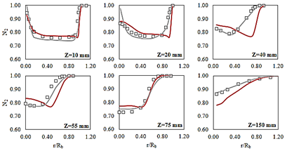
Fig. 15 shows a wide difference between the experimental data and RANS results for the radial samples of temperature and CO 2 mass fraction, taken at z = 10 mm and z = 20 mm. The experimental data suggests no presence of such temperature peak behind the bluff body. Meanwhile, results from the LES simulation fairly agree with experimental data in this matter.
Source: The authors.
Figure 15 Profiles of time-averaged temperature, mean temperature, mean H2O mass fraction and mean CO2 mass fraction for experimental data (squares), RANS (grey line) and LES simulations (red line)
The general shape of the flame neck is successfully captured by the two turbulence models. However, it can be realized from species mean mass fraction and temperature profiles, shown on Figs. 15-16, that RANS model results do not qualitatively match to the experimental data.
Source: The authors.
Figure 16 Profiles of mean N2 mass fraction for experimental data (squares), RANS (grey line) and LES simulations (red line).
Radial samples taken at z = 40 mm and z = 55 mm for the LES simulation results shown that the peck of temperature and species mass fraction is displaced closer to the combustor center-line than experimental data shown. Additionally, the temperature peck on the neck edge is overestimated by both models. The displacement of the profiles and the temperature overestimation, for those radial samples, is a comprehensible behavior considering the overestimation of 15 mm downstream of the flame neck location.
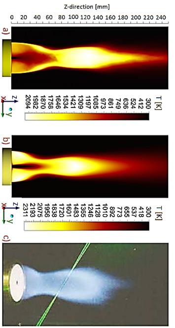
Another important consideration is that the maximum temperature recorded during the experiments was 1928 𝐾, located at the axial position of 75 mm downstream and radially located at 2 mm from the combustor center-line (Z = 75 mm and r ⁄ R B = 0.08). Fig. 17 shows contours of time-averaged temperature (LES model), mean temperature (RANS model) and a photograph of temperature field captured during SMA1-flame test. As can be appreciated from Fig. 17a, temperature field over the BRZ is spatially overestimated, covering a larger zone than SMA1-flame photograph shown, Fig. 17c.
Source: The authors for figure 17.a and 17.b; figure 17c was taken from 39.
Figure 17 Temperature contours: a) time-averaged temperature, b) mean temperature (RANS model) and c) a photograph of SMA1-flame.
This behaviour is mostly induced by the wrong neck location estimated by the LES model. On the other hand, Fig. 17b shows a spatial underestimation of the temperature field on the BRZ. The low jet’s decay rate and the high mixing rate have reduced the high temperature reaction zone, appearing a narrow flame neck, a stronger recirculation zone behind bluff body and a temperature peck closer to the bluff body than experimental observations suggest. The simulation results shown that the zones with the highest temperature peak appear at Z = 100 mm and Z = 120 mm for the RANS (2311 K) and LES (2094 K) models, respectively. The experimental observations of the SMA1-flame suggest that the flame length extends until Z = 120 mm.
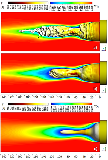
From the numerical results could be estimated the flame length, based on the stoichiometry oxygen mass fraction distribution. The estimation is made considering the edges of the visible part of the flame as the stoichiometric surfaces, where the main reactions are taken places 40. Fig. 18a shows the time-averaged contours of 𝑂 2 mass fraction with imposed instantaneous iso-surfaces at stoichiometric 𝑂 2 mass fraction, colored by temperature. The figure shows how a typical flame shape look like. In this work 30000 time-steps are consider for carrying out time-averaged of the interest magnitudes. Fig. 18b shows the time-averaged contours of 𝑂 2 mass fraction with imposed time-averaged iso-surfaces at stoichiometric 𝑂 2 mass fraction, colored by temperature. From the figure could be noticed that LES results showed a flame length overestimation in about 10 mm. Fig. 18c showed that the flame is 20 mm shorter than experimental observations suggest for the RANS case. The two recirculation zones act as two opposite dynamic forces, stretching the flame and shaping itself. Therefore, flame features such as length, neck location and the mixing process in the shear layer are strongly conditioned by the capability of the turbulence model for capturing and accurately represent those two recirculation zones.
Source: The authors.
Figure 18 Contour of O2 mass fraction with imposed iso-surface at stoichiometric O2 mass fraction colored by temperature: a) LES results with instantaneous iso-surface at stoichiometric O2 mass fraction, b) LES results with time-averaged iso-surface at stoichiometric O2 mass fraction and c) RANS results with mean iso-surface at stoichiometric O2 mass fraction.
5. Conclusions
The mesh resolution of the LES was shown to be a key matter in the application of this turbulence modeling approach, where critical regions should maintain adequate mesh resolution and the highest possible quality. LES with Dynamic Smagorisky-Lilly sub-grid model was capable of capturing the main flow features, but the central jet’s decay rate was not accurately predicted. Being observed a high mean deviation for the time-averaged axial-velocity at jet’ centerline for radial samples taken at 20 mm, 40 mm and 60 mm downstream. The EDM in combination with the LES turbulence modeling approach showed a reasonable performance in terms of species and temperature profiles accuracy, considering the simplified chemistry handled by the EDM. In general, near wall resolution, time and spatial resolution should be carefully assessed to obtain physically reliable results from a LES turbulence modeling approach

