


 Inglés (pdf)
 Articulo en XML
 Referencias del artículo
 Enviar articulo por email
 Citado por SciELO
  Citado por Google
  Similares en
SciELO
Similares en
SciELO  Similares en Google
 Permalink
1. Introduction
The environmental processes of the urban atmosphere refer to that lowest portion of the troposphere with a thickness varying, between day and night, from a few kilometers to a few hundred meters. In this atmospheric layer, the ground and the troposphere heat exchanges are responsible for the region's most characteristic dynamic and thermodynamic processes. Additionally, the anthropic impacts can modify the local climate and air quality of its depth [1]. This region is known as the Atmospheric Boundary Layer (ABL), and Stull (1988), a classical author on the subject, defines it as "that part of the atmosphere that is directly influenced by the presence of the earth's surface, and responds to surface forcing with a timescale of about an hour or less [1]. By forcing refers to processes such as evaporation, transpiration, the drag effects produced by the wind, heat transfers, changes in use and land cover, and emissions of pollutants.
The ABL develops, between terrain and the upper free atmosphere (FA), enough quantity of turbulent kinetic energy (TKE) [1-4] to transport momentum, energy, chemical species, and pollution in its full extension. However, the origin of daytime TKE is related to the radiative energy of the sun heating the earth's surface, while nighttime TKE comes mainly from low-level jets (LLJ) near the ground. Thus, the daytime ABL is called the Convective Mixed Layer (CML), with the Mixed Layer (ML) as a portion of it, where the TKE is substantial, and the Nocturnal Boundary Layer (NBL), mainly a stable stratified layer, above which there is a relatively quiet residual layer (RL) that occupies the remaining space of what was just a few hours before the ML [2,5-7].
In other words, during the day, solar heats the land surface, activating positive heat fluxes and creating atmospheric instability with a negative vertical temperature gradient, the ML expands within the ABL; meanwhile, above the ML remains a thermal inversion layer (IL) characterized by a positive vertical temperature gradient, which inhibits the mixing of air parcels. In contrast, at night, as the radiative fluxes cool the land surface, it forms a surface inversion layer (SIL) with a severe stable temperature gradient at the base of the atmosphere, above which develops the NBL, where the LLJs produce turbulence [1,4-6] (Fig. 1).
Within the ABL, approximately 10% of its total height is occupied by a surface layer (SL), which plays a crucial role in exchanging momentum, heat, and pollutants between the earth's surface and the ABL in urban regions. The SL represents a heterogeneous region characterized by urban structures such as buildings, roads and vegetation that interacts with the thermal and turbulent flows, creating distinct airflow patterns [1,7,8].
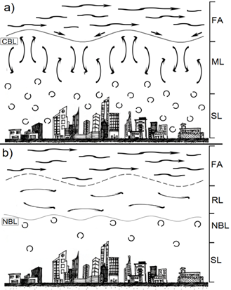
Source: Own elaboration and adapted from [8].
Figure 1 Circulation schemes a) CBL and b) NBL. Eddies represents thermal and turbulent flows. The right margin of each image displays the distinct layers comprising the CBL and NBL.
Research on low-level nocturnal circulation has been conducted using theoretical and numerical models, which rely on physical and thermodynamic variables [9,10]. Some of these studies have highlighted the importance of the interactions between terrain heterogeneity and atmospheric processes, such as radiative cooling and orographic drag [11-13]. For instance, the presence of clouds can affect atmospheric stability, with clear skies and weak winds promoting strong NBL stability and weak turbulent flows; in contrast, low cloudiness and high winds weaken stability and promote continuous turbulent flows. Besides that, the Gravity currents cool the surface atmosphere and warm air at altitude, creating cold air pools that affect atmospheric stratification. Meanwhile, the nocturnal heat islands in urban areas have been shown to weaken atmospheric stratification [11,14-22].
This research aims to characterize the thermal and dynamic structure of the NBL in the Aburrá Valley (AV). This valley is a tropical urban area of complex topography located in the center-western of Colombia, coordinates N 6.15° - W 75.30°, in the foothills of the central mountain range of the Colombian Andes; where the alignment of the river broadly follows the direction South-North, although its trajectory is a broken line with various direction changes. In the most urbanized zone, the valley's base is at an altitude of about 1,500 meters and rises at some points to just over 3,000 meters above sea level. Although the higher distance between the opposite peaks of the valley reaches up to 20 km, it predominates 10 km between them, for which many authors refer to it as a moderately deep valley.
Due to the accelerated demographic and vehicular growth in AV, high concentrations of particulate matter (PM) and other atmospheric pollutants have gained attention as an urban environmental problem. Furthermore, although local air quality management policies have contributed to improving the situation, they surge several worries about the need for knowledge about some atmospheric processes in the territory and the potential impacts of pollution on the health of people and the surrounding ecosystems.
Research on meteorological processes and air quality in the AV shows evident advances over the last 20 years, both from the point of view of monitoring and measuring variables in the ABL, as well as in the incorporation of numerical models more versatile and sophisticated (e.g., WRF, HYSPLIT, ENVI-Met) that have allowed a better understanding of atmospheric dynamics and urban pollution problems in this metropolitan area. For example, with the support of the Sistema de Alerta Temprana del Valle de Aburrá (SIATA), [23,24] characterized the structure of the ABL during the daily cycle to estimate its thickness and understand how the ABL behavior affects the concentration of urban air pollutants. In the same line, [25] studied local processes of soil-atmosphere interaction and their relationships with meteorological conditions, while [26] analyzed the connections between atmospheric dynamics in the VA and the concentration of urban pollutants at regional and local scales.
In general, the air quality concerns in the AV revolve around the ML performance since the events with the highest concentration of particulate matter usually occur in transitions from night to daytime hours or, on the contrary, from the daily to nighttime hours, except for the longer contingency of several days, as has been the case in March, every year since 2016 [28]. Thus, here we ask about the thickness of NBL in the AV, its evolution patterns throughout the night and over the year, and about a reliable method to estimate its thickness. This research is based on 2017 data from remote sensing meteorological equipment managed by SIATA. The methods and results in this article correspond to those selected and obtained by [29-30] in his master's dissertation.
2. Methodology
This section presents the databases used in this research and our treatment to explore the nocturnal atmospheric processes of AV. It characterizes the atmospheric processes at night and introduces the critical BRN criteria.
The meteorological data utilized were sourced from SIATA, an organization responsible for monitoring various hydro-meteorological variables that could potentially lead to environmental hazards in AV. Fig. 2 highlights the locations of two essential sensors, the Radar Wind Profiler (RWP), and the Microwave Radiometer (MWR), both of which are positioned within the urban zone of AV at the base of the valley. Given their significance, it is imperative to include these sensors in the document for comprehensive analysis.
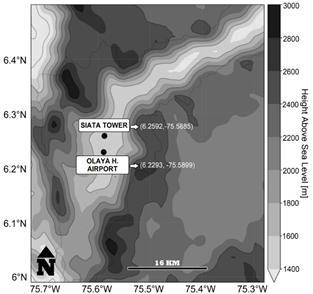
Source: Own elaboration.
Figure 2 Remote sensor locations. CL and RM in SIATA Tower and RWP in the Olaya Herrera Airport.
The RWP is a Raptor Velocity-Azimuth Display Boundary Layer (VAD-BL). This facility operates in The Olaya Herrera Airport, 5 km south of SIATA tower. This sensor estimates the wind components (µ,ν,ω) from 77 m to 8.000 m, with a temporal resolution of 5 min. The whole record for the year 2017 is available.
The MR (model MP-3000A) is located at the border of the sporting center of Medellin city, at the terrace of SIATA Tower, about 50 m over the ground. It gets vertical profile information of temperature, relative humidity, liquid density, and water vapor density, from 50 m to 10.000 m, with a time resolution of 2,2 min. Additionally, this sensor measures atmospheric pressure at the sensor level. The record for the year 2017, except for January, is available.
The Vaisala ceilometer (CL, model CL-51) is also located in the SIATA Tower, next to the MR sensor. This instrument provides information about clouds, aerosols, and particles in the atmosphere based on a pulse laser operating at a near-infrared wavelength (910 nm). Pulse-laser signal backscatters at different altitudes depending on the particulate elements encountered on its path. It operates with a spatial resolution of 10 m up to 15.000 m, with a temporal resolution of 16 s. The record for the year 2017, except for December, is available.
2.1. Data processing
The primary goal of the data processing was to estimate the state variables of nighttime atmospheric phenomena and evaluate various NBL thickness methods. The initial step involved standardizing the databases through linear temporal and spatial interpolation of MR, RWP, and CL records. This led to a set of uniform data series at 5-minute intervals, with a consistent resolution of every 50 meters (e.g., 150m, 200m, 250m). As a result, the processed data provided a reliable foundation for testing the NBL thickness methods under investigation.
The Specific Humidity (SH) [g kg-1], virtual potential temperature (θv) [K], the horizontal wind direction and velocity [° and ms-1], backscatter intensity (BS) [10-9m-1 sr-1] and BRN. The equations that govern these variables are described in several texts, mainly referenced in [1,4,31].
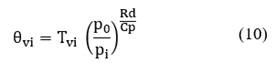
For instance, to estimate the θv at some i-height, it is necessary to calculate the corresponding potential temperature (θ) with eq. (1):
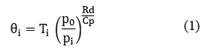
Where T represents the absolute temperature, Rd is the gas constant for dry air, Cp is the air-specific heat at constant pressure, and p0 is the usual reference pressure (1000 hPa).
Because MR only reports the lowest level pressure, it is necessary to use the hypsometric eq. (2) to compute the pressure at other z-levels:
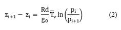
Then, we obtain eq. (3):
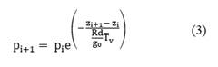
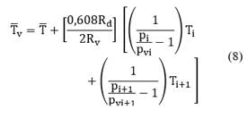
Here zi and pi are the i-eight and the i-pressure, g0 is the gravity acceleration and
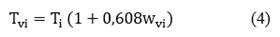
 is the average virtual temperature between i and i + 1. Levels. Thus, Tv results from eq. (4):
The vapor mixing ratio, wvi, is calculated by eq. (5):
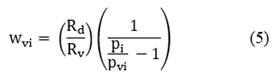
Where Rv is the water vapor constant, pv is the water vapor pressure and pd is the dry air pressure. Therefore, to estimate pv eq. (6), we need to estimate the saturation vapor pressure pvs eq. (7):
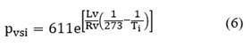
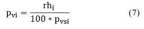
In eq. (6)-(7), Lv is the latent heat of evaporation, and rh is the relative humidity. Here,
corresponds to the expression:
And pi + 1 to:
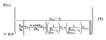
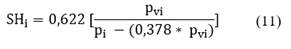
To estimate the magnitude of pi + 1 is necessary to use a numerical method, such as Newton-Raphson. Then, having calculated the p at some i-level, it is possible to estimate θv and SH from the eq (10)-(11):
Finally, using the θv and the wind record coming from the RWP, the BRN corresponds to the eq (12) [4]:
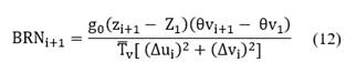
In this case, u and v are the zonal (along latitudinal lines) and meridional (along meridian lines) wind components. Because the MR and RWP operate in different sites with slightly different altitudes, this condition may generate biases in BRN estimation.
2.2. Data exploratory analysis
To estimate the NBL thickness was necessary to analyze the NBL structure, checking its behavior through different methods, including the BRN vertical profiles. The evaluation of NBL thickness error for each method requires a reference thickness value provided by the ceilometer as the Minimum Backscattering Gradient (MBG) due to its demonstrated reliability corroborated in the context of previous research for AV [24]. Hence, the Root Mean Square Error (RMSE) is defined by eq. (13):
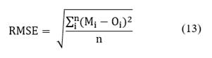
Where Oi represents the NBL thicknesses estimated by MBG and Mi is the corresponding NBL thicknesses deduced from some other specific method.
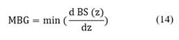
The signal intensities provided by CL sensors depend on the types of particles that backscatter light in the atmosphere due to the presence of water vapor, aerosols, and particles. These substances are mixed by turbulent diffusion, creating a thick layer over the NBL that inhibits mass transport into the free atmosphere [13]. The minimum gradient of the BS in the profile represents the NBL thickness by eq. (14):
Another standard method is the Non-local Thermal Inversion (NLTI). It consists of evaluating the static stability to delimit the SIL thickness. Typically, the SIL is the region with a positive slope [32-36]. Over the SIL, there may be atmospheric instability layers (negative slope) or neutral conditions (undefined slope). Then, NLTI is the combined thickness of SIL and its contiguous layer, which can be either unstable or neutral [2]. The minimum gradient θ vi in the profiles provide an NBL thickness computed by eq. (15):
The atmospheric cooling may impact aerosol size due to hygroscopic effects, increasing low-level cloudiness [37]. SH profile at night is commonly negatively sloped, and as the height increases, it exhibits gradients associated with condensation effects and atmospheric stratification [38]. The minimum gradient in the profile is a potential signal of NBL-thickness, calculated by eq. (16):
The LLJ corresponds to a maximum wind velocity close to the earth's surface, contributing to shear effects and atmospheric transport of substances [1,39-41]. Given the presence of multiple local maxima in the wind velocity profile, we consider the highest gradient of wind velocity within the initial 650 m as indicative of the LLJ:
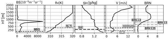
Source: Own elaboration.
Figure 3 The estimates (dotted lines) of the NBL thickness according to the vertical profiles of backscatter intensity (BS), virtual potential temperature ( θ v ), specific humidity (SH), wind velocity (V), and Bulk Richardson Number (BRN) methods.
An alternate technique identifies the minimal wind velocity gradient within the initial 650 m, capturing the turbulence-reduced lower troposphere [42-44]. This thickness is computed using eq. (18).
The dimensionless Richardson number (Ri) considers the relationship between the TKE generated by buoyancy effects (thermal forces) and shear effects (mechanical forces), simplifying the analysis of turbulent flow. The BRN formulation is the Ri finite difference parameterization, defined in eq. (12).
The critical BRN (CBRN) represents the level where turbulent flows weaken, with a value of 0,25 based on linear stability theory. However, for nonlinear stability theory, a more suitable value is 1,0 [11, 45]. According to this criterion, BRN < 1 represents turbulent flow, while BRN > 1 stands for laminar flow. Controlled experiments, atmospheric models, and observations have shown CBRN ranging from 0,1 to 7,2 [9]. Thus, a universal CBRN does not exist due to TKE depends on physical processes and surface/terrain characteristics [46-50].
Fig. 3 depicts vertical variable profiles illustrating the application of each method in determining NBL thickness.
3. Results
3.1. Data processing
In this numeral, wind, θv, BS, and BRN profiles were analyzed to discern nocturnal atmospheric patterns and processes in both dry (DJF - JJA) and rainy (MAM - SON) quarters, utilizing quarterly hourly averages within the range of 50 m to 2800 m. By choosing these altitude levels, it allows enables the identification of significant local and mesoscale characteristics and their correlations.
3.1.1. Wind
Fig. 4 shows the quarterly hourly average of wind direction. The average wind regime contrasts drastically during the year across z~1150 m. Under this level, northeasterly orographic winds dominate; but above it, over the surrounding peaks of the AV, the Trade winds tend to impose the circulation patterns.
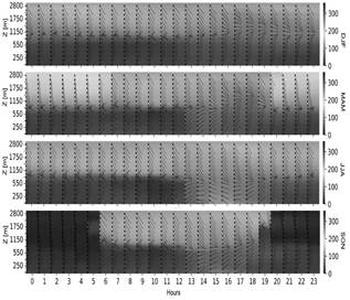
It is remarkable that in the SON quarter, some coupling of winds at night occurs, which results in the cancellation of shear effects along the local-mesoscale night wind contact surface. This quarter shows how the upper winds change direction between daytime and nighttime. Because the Trade winds do not substantially change their direction between day and night, the local wind seems to drag some of the air above it; and this could be possible because Trade winds during SON quarter are light.
In contrast, in the MAM, JJA, and DJF quarters, the presence of shear effects in the contact surface during nighttime hours is evident. Furthermore, Fig. 4 shows no changes in the valley wind direction between day and night, contrary to the classical theory, which talks about down-valley winds at night; this is likely a consequence of the presence of surface hot spots at the south of VA (up-valley urban island). By the way, it is notable that in the JJA quarter, By the way, it is notable that in the JJA quarter, directional coupling occurs during daytime hours.
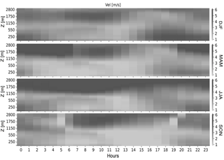
Fig. 5 represents the quarterly hourly average wind velocity and reveals the development of LLJ at the most superficial atmospheric levels during nighttime. The LLJ attains its peak between late evening and midnight, vanishing prior to sunrise. Specifically, in the DJF and JJA quarters (dry periods), LLJ develops before sunset, averaging about ~4 m/s with mean thicknesses of 500 m. Conversely, in the MAM and SON quarters (rainy periods), LLJ develops after sunset, with lower velocity of ~3 m/s and mean thicknesses ~300 m. Notably, the LLJ in the MAM quarter is characterized by weaker velocities, lower thicknesses, and shorter overnight lifetimes.
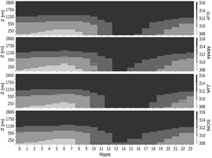
3.1.2. Virtual potential temperature
Fig. 6 shows the quarterly hourly average of the θ𝑣. During sunny hours, the DJF and MAM quarters exhibit cooler surface levels compared to the JJA and SON quarters. This aligns with a weak expansion of convective boundary layers and the occurrence of pollution episodes in AV during March and November. Some researchers link the persistent high levels of particulate matter in the boundary layer during March to the prolonged presence of cloudiness without rain throughout the day and the reduced irradiance conditions in this month, attributable to the Intertropical Convergence Zone's relatively distant position [51].
Across the four quarters, θ𝑣 profile thermal inversion is generally observed at night, making NBL thermal stability stronger during the rainy quarters. Among these, the MAM quarter displays the strongest stability, attributed to consistent cloud cover throughout the day and fewer variations in irradiance during this period.
Backscatter
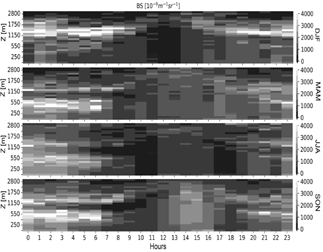
Fig. 7 shows the quarterly hourly average of BS, where values greater than 1000 [10-9m-1 sr-1] indicate the presence of clouds, aerosols, and particles [23]. Lower BS concentrations during sunny hours primarily result from vertical mixing driven by the ML's expansion, facilitating particle transport from the surface to the free atmosphere.
Conversely, notable BS concentration escalation is observed at night, particularly from midnight to sunrise, attributed to the accumulation of particles close to the surface. This rise is influenced by static stability, intensifying pollution, and water condensation at lower atmospheric levels.
On the other hand, the seasonal BS variations confirm the less favorable circumstances to mix and transport particulate matter in AV during MAM and SON quarters compared to the JJA and DJF quarters.
Bulk Richardson Number
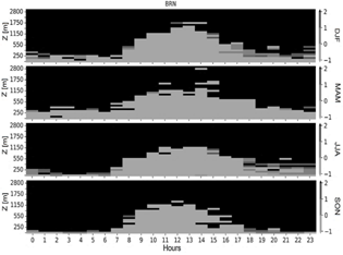
Fig. 8 illustrates the quarterly hourly average of BRN. Following sunrise, a layer with low or negative BRN extends up to and beyond z~1150 m across all four quarters, denoting elevated atmospheric turbulence. However, as sunset approaches, the turbulent layer gradually dissipates, and the boundary layer transitions to higher BRN values, indicating the development of dynamic stability.
At altitudes below 400 m during nighttime, the BRNs are comparatively lower in the DJF - MAM period than in the JJA - SON period, with the SON quarter showing the highest values. This behavior suggests that the JJA - SON quarters exhibit a stronger superficial static nocturnal stability, coherent with numeral 3.1.2.
NBL Structure characterization
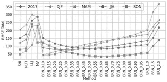
As previously mentioned, the MBG method serves to estimate nighttime CBRN (18 h - 6 h) by assessing RMSE of hourly medians in comparison with other methods. Fig. 9 shows that the RMSE of the BRN method varies by semester, with the DJF - MAM period shows lowest RMSEs around BRN values near 0,1, while the JJA - SON period displays its lowest RMSEs for BRN values between 0,5 to 0,6. Furthermore, the figure highlights the relatively favorable performance of the SHI and NLTI methods during rainy quarters, notable for their practical applicability in estimating NBL thicknesses and aligning with the quarters with more significant air quality concerns in the AV.
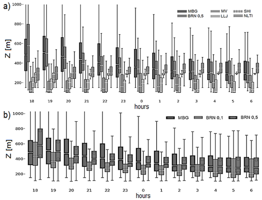
The hourly trend of the thickness for MBG, BRN, and other methods provides deeper insights into the NBL's thermal and dynamic evolution. In line with this objective, Fig. 10.a depicts NBL thickness estimates and their changes throughout the night using six methods, including the approach based on CBRN of 0,5.
The Fig 10.a illustrates that the LLJ hourly median reflects a decreasing estimation of NBL thickness, reaching its peak local value around z~200 m at 18 h and z~130 m by 6 h. Conversely, the MV method exhibits an increasing estimation of NBL thickness, with the minimum local value evolving from z~120 m at 18 h to z~210 m towards the late-night hours. Certainly, the NBL estimations from both methods mirror the patterns observed in the nocturnal wind data. Dring dusk, surface winds are weak, while slightly higher velocities are recorded around 200 m above ground level. As the night advances, stronger winds tend to be closer to the surface; meanwhile, a minimum velocity wind gradient gently moves up along the night. Nevertheless, it's worth noting that the LLJ and MV methods consistently yield underestimations of NBL thickness across all cases when compared to the estimates obtained from the MBG method.
Source: Own elaboration.
Figure 9 The hourly median RMSE of the NBL thickness to the listed methods against the MBG reference method for the seasonal quarters DJF, MAM, JJA, and SON, during 2017.
The SHI and NLTI s demonstrate a tendency to amplify NBL thickness estimations throughout the night. Specifically, the SHI method identifies condensation levels localized at approximately z~260 m at 18 h and z~300 m at 6 h. In contrast, the NLTI method indicates a minimum of the virtual potential temperature that evolves from about z~300 m at sunset to z~350 m at sunrise. Although these methods exhibit slight variations in NBL thickness estimations over the night, they lean towards underestimating this parameter, particularly prior to midnight, in comparison to the MBG approach.
Before considering the BRN results, a natural question arises from Fig. 9: In the context of AV, which CBRN value, annual or semestral, is more suitable for evaluating NBL thickness? Fig.10.b, derived from 2017 data, offers some insight into this matter: the BRN method with CBRN set at 0,1 consistently leads to underestimated NBL thickness, while with CBRN set at 0,5, the medians of MBG and BRN closely converge. Both series exhibit a declining trend throughout the night, initiating from a median z~500 m to z~600 m and gradually decreasing up to sunrise, approximating a thickness of z~300 m. Going back to a Fig. 10.b, the behavior of CBRN 0,5 closely mirrors the MBG median and reflects dispersion patterns.
4. Discussion
Between the six more common methods proposed by technical literature to estimate the thickness of the NBL in AV, we assumed the MBG as the reference. This choice is based on a reliable set of previous research, fed by trusted data collected primarily during the last decade.
It is worth saying that although the methods based on SHI, NLTI, MV and LLJ do not provide fitted estimates of NBL thickness of AV, they give some insight into its NBL characteristics. By performing an hourly sensitivity analysis, it is possible to gain a more detailed understanding of the thermal and dynamic structure of the NBL. This analysis focuses on two key factors: the deficit in all-wave surface radiation during the short night, leading to surface cooling, and localized turbulent flows near the upper NBL. These turbulent flows are influenced by the collapse of ABL convective processes and shear effects induced by LLJ. The study reveals rapid transformations of the ABL in the dusk, resulting in the formation of an aloft RL and a deeper SIL as the night progresses. Prior to sunrise, the prevailing stable atmospheric conditions contribute to a light LLJ, resulting in weaker turbulent flows and pollutant dispersion.
Indeed, the LLJ is a crucial factor in the dynamics of turbulent night flows, acting at night as the primary agent for the transport and dispersion of pollutants in interaction with Trade Winds. The effects discussed can be better understood by referring to Fig. 11, which depicts the NBL structure at 19 h, 0 h, and 5 h.
Source: Own elaboration.
Figure 10 Evolution of the NBL median and dispersion thickness during 2017. a) MBG, MV, SHI, BRN=0,5, LLJ and NLTI methods b) MBG, BRN=0,1, and BRN=0,5 methods.

Source: Own elaboration.
Figure 11 Representation of the thermal and dynamic structure of the NBL over the VA at a) 19 h, b) 0 h, and c) 5 h. Each frame illustrates the profile of 𝜃𝑣, the TKE by eddies, the SHI by a dashed line, and the LLJ by the height and length of the arrows. As the night advances, the cooling effect intensifies (∂θv /∂t<0).
Notably, the local night winds and the LLJ blow consistently in the up-valley direction of AV, which contradicts the traditional theory of down-valley mountain winds at the matured night [52]. This fact could result from surface hot spots in the valley's south, creating an up-valley urban island which, nevertheless evidence, deserves more research.
Many authors refer to the BRN method as one of the most convenient to estimate the evolution of NBL thickness. By using virtual potential temperature data and wind velocity measurements at various altitudes, we integrate this information to compute the BRN. Through this approach, we can determine the CBRN, which correlates with the thickness of the NBL. For the case of AV, the nighttime CBRN was derived by testing BRN values ranging from 0,1 to 2,0 for delimiting the NBL and comparing them with MBG thickness estimations through RMSE metrics. A CBRN equal to 0,5 was identified as closely aligning with MBG estimations for the year 2017. This CBRN is consistent with values referenced in other NBL stability studies worldwide, the majority below 1,0 [9]. However, studies conducted by other authors in the AV suggested that CBRN are closer to 4,0, a significant difference that could be attributed to the use of different BRN formulas and different periods focused on.
The atmospheric conditions in the different quarters of the year give us additional information about the NBL behavior. In AV, during 2017, the NBL for the DJF and MAM quarters (Northern winter and spring) were more statically stable than JJA and SON ones, while JJA and SON quarters (Northern summer and fall) were more dynamically stable, occurring the most intense dynamic stability events during the SON quarter. On average, the top of NBL was located around 250 m over the ground during MAM and DJF quarters, while it was around 150 m during JJA and SON quarters.
On the other hand, LLJ tends to have lower velocity and thickness during rainy periods (the MAM and SON quarters) and exhibits reduced mechanical effects due to early turbulent dissipation. In contrast, a thicker and longer LLJ is typically observed during dry periods (DJF and JJA quarters) and can persist for several hours after sunrise, as seen in the DJF quarter.
In terms of nighttime air quality, the JJA and SON quarters conditions contribute to an enhanced dynamic stability regime and reduction in the thickness of NBL. Nevertheless, due to the atmospheric stability during the daytime, MAM quarter usually exhibits higher records of pollutant concentrations throughout the diurnal cycle. In any case, the NBL in AV experiences relatively high wind velocities earlier at night, and near-zero wind velocities after midnight, enhancing the potential risk for a pollution episode due to the NBL, typically with a thickness ranging between 200 m and 300 m.
Thus, it is interesting to pay attention to the suggestions from some administrative and environmental regional authorities to privilege the transport and operation of heavy loads vehicles (such as trucks and dumpers) during nighttime, arguing the possibilities to improve mobility in the AV, repeatedly mentioned in recent years. However, as revealed by this study, such actions could adversely affect air quality due to the significant pollutant load released by these vehicles, which accounted for approximately 66% of the total PM 2,5 emissions in 2018 [53].
Even more, during the day, people seem to be more conscious of pollution in the AV due to the more visible presence of airborne particulates. However, the smog layer at night may be unnoticed, and people may not be as concerned about it, potentially leading to a false sense of security. Additionally, the potential implications of a critical pollution episode at night remain unclear, and the chemical and physical processes of pollutants during nighttime hours in the AV still need to be well understood. Therefore, AV's air quality management system must promptly mitigate harmful effects arising from nocturnal meteorological conditions and pollution emissions. It should also be prepared to address potential episodes of nighttime pollutants, posing health and ecological risks in the region.

