


 English (pdf)
 Article in xml format
 Article references
 Send this article by e-mail
 Cited by SciELO
  Cited by Google
  Similars in
SciELO
Similars in
SciELO  Similars in Google
 Permalink
1. Introduction
Research in algorithms for the optimal reconfiguration of radial distribution systems is always present in the specialized bibliography. Extensive reviews like Mishra’s [1], Sultana [2] or Mahdavi [3] present hundreds of contributions.
The heuristic branch-exchange algorithms for the distribution systems reconfiguration of Cinvalar [4] and Baran [5] are based on the interchange of the system’s open branches to obtain the minimal losses radial configuration that can supply the load at required voltage. Goswami [6] introduces the concept of optimal flow pattern to simplify the determination of the branch to open in a closed loop, while Nara [7] formalizes the single-stage branch-exchange algorithm as well as the multi-stage branch exchange algorithm. In addition, Abul’Wafa [8] presents an efficient implementation of the branch-exchange method.
In other line of thought, first Shirmohammadi [9] and late Gomes [10] propose a heuristic that starts analyzing a meshed distribution system which switches are open successively until eliminate the loops and obtain the optimal radial configuration.
Different types of meta-heuristic methods are applied in reconfiguration. Ching-Tzong Su [11] uses an improved mixed-integer hybrid differential evolution method to reduce power losses and enhance the voltage profile by system reconfiguration. Das [12] presents an algorithm based on heuristic rules and fuzzy multi-objective approach that considers load balancing among the feeders, power losses, deviation of nodes voltage, and branch current constraints violation. In addition, Abdelaziz [13] proposes a modified particle swarm optimization (PSO) algorithm. Souza [14] [15] presents a very efficient artificial immune algorithm applied to distribution system reconfiguration with fixed or variable demand.
There are many contributions to reconfiguration based in genetic algorithms. The binary coded chromosome of Nara [16] represents the on/off status of all system branches. As unfeasible solutions can appear, Ramaswamy [17] applies repeatedly genetic operations until the obtaining of feasible individuals is achieved. Their implementation of the non-dominated sorting genetic algorithm (NSGA-II) minimizes power loss, voltage deviations, current deviations, etc. In addition, Tomoiagă [18] uses NSGA-II as well for optimizing losses and reliability indexes.
Sahoo [19] uses a binary coded genetic algorithm for minimizing voltage stability factors, each tie branch is represented in chromosome by a binary substring that determines the branch to open for maintaining the radial configuration. Vitorino [20] utilizes the same codification. In addition, Hsu [21] employ NSGA-II, using a source zone encoding method to reduce the possible appearing of illegal chromosomes during reproduction.
The genetic algorithm presented by Mendoza [22], utilizes a new codification strategy and novel genetic operators, called accentuated crossover and directed mutation. The method begins by identifying the fundamental loop vectors of the system’s graph. The fact that only one branch can be open in each fundamental loop vector, simplifies the codification of chromosome, which represents the open branches by decimal integers. This improved technique can produce non-radial topologies, so, especial genetic operators complement the method to correct this. Even with that technique, infeasible individuals appear. In the same direction, Gupta [23] uses fundamental loop vectors to generate feasible individuals. In addition, he introduce common branch vectors and prohibited group vectors with rules that avoid the generation of infeasible individuals. Zidan [24] and Eldurssi [25] employ both the Gupta's codification. The difficulty of the method is the huge amount of prohibitive group vectors that appear in large circuits.
In another direction, Carreno [26] implements a genetic algorithm which chromosome represents both: the closed and the open branches. In each step, only one descendent is generated using the selection, recombination, mutation and local improvement sequence based on the branch-exchange technique. Madhavi [3] uses a similar codification and local improvement in their efficient genetic algorithm contribution.
As can be seen in literature, many heuristics for network reconfiguration rely on the systematic applying of the branch-exchange technique. In this work are developed two novel genetic operators for crossover and mutation that are based on the branch-exchange technique. The chromosome's codification to use these operators is straightforward and is not required any additional knowledge of graph theory to achieve the feasibility of individuals.
As one of their main novelties, the methodology shows how can be employed a local improvement step, used commonly in the single-objective optimization, in the multi-objective optimization. This step increases the convergence of the optimization with populations of much reduced size. The proposed methodology is tested by solving several examples of the literature, including or not the local improvement step. The comparison of the results with the best solutions published for these examples shows the effectiveness of the method.
2. Problem formulation
In essence, most of the formulations for the reconfiguration problem consider the minimization of losses as the objective function to minimize. Although other objective functions can be selected, the present work formulates reconfiguration as a multi-objective optimization problem that minimize system losses cost and voltage deviations in the load nodes. The solutions are subject to be feasible radial configurations.
2.1. Independent variables
The independent variables of the problem, represented by the array x, are the set of branches that must be open to obtain the radial circuit with optimal configuration respect to objective functions. For a meshed network of N nodes and M branches, the number of branches to be open to obtain a radial configuration is equal to L.
2.2. Constraints
The main constraint to this problem is that any solution of reconfiguration must represent a radial circuit. The fulfillment of this apparently simple constraint is one of the main difficulties in the solving of reconfiguration problem with any optimization method.
2.3. Objective functions
Several objective functions can be considered for the presented problem. This work considers two objective functions: minimum system losses cost (f1) and voltage deviations (f2) at load nodes.
System losses cost in network conductors is calculated for 24h variable daily demand with variable costs of energy ck ($/kWh) at the different k-hours as:
Where ΔPk(x) is the network power losses at hour k.
On the other hand, the minimization of voltage deviations at load nodes is achieved by minimizing the maximum voltage deviation respect to the source among all i-nodes and the k-hours.

The determination of the voltages and the power losses at different load states is achieved by using a forward-backward sweep power flow.
3. Optimization algorithm
NSGA-II is one of the methods of more success in multi-objective optimization. Like every genetic algorithm, the solving of a particular problem by the NSGA-II implies some adaptations and the programming of certain parts of the algorithm. In this case, a NSGA-II implemented in Matlab [27] is adapted for the solving of the presented problem.
A solution of the reconfiguration problem is described by the set of open branches in the network. Thus, the chromosome is composed by an array of L integer values, which represent the indexes of the open branches.
In order to obtain feasible radial configurations, the presented implementation of NSGA-II employs the technique of exchange of branches. That is, the change of the gene k in chromosome for a gene j that does not belong chromosome implies the closing in the circuit of the branch k and the opening of the branch j. This branch-exchange technique assures the circuit remains radial.
Two genetic operators of crossover and mutation are developed in this work that applies the cited technique. The offspring of these operators is always a feasible radial circuit. In the presented implementation, an 80% of the offspring is generate by crossover and the remaining 20% is obtained by mutation of population.
Optionally, the implemented algorithm includes a local improvement step, which is applied after the genetic operations of crossover and mutation.
3.1. Crossover operator
The crossover operator determines the offspring c1 and c2 by interchanging a random subset u of genes between the chromosomes p1 and p2 of both parents, element to element. The process must guarantee that offspring chromosomes maintain the feasibility, that is, they must represent radial configurations of the circuit. However, due to the characteristics of the problem, is very rare that feasible offspring’s c1 and c2 be obtained with this technique.
The extraction of a gene p1(k) from chromosome p1 implies that branch p1(k) close, which forms a loop in the circuit. To retrieve the radial configuration, a branch belonging to the loop must open. This procedure assure the obtaining of feasible offspring chromosomes.
After several tests, the implemented crossover operator works as follows. If branch p2(k) belongs to loop (about 3-5% of cases), then the branch p1(k) is substituted by branch p2(k), otherwise, the branch p1(k) is substituted by mutation, selecting at random one of the branches adjacent to p1(k) in the loop. The following steps illustrate the procedure:
1) Finds the loop created by closing p1(k) in the circuit.
2) If branch p2(k) belongs to loop, loop(j) = p2(k). Otherwise, selects at random the branch loop(j) as one of the branches adjacent to p1(k) in the loop.
3) Close the branch p1(k) and open the branch loop(j) in the circuit.
4) The gene p1(k) is substituted by gene loop(j)
Once all the selected genes p1(u) are substituted in chromosome p1 (up to 10% of genes), the offspring c1 is equal to the changed p1 vector. The offspring c2 is obtained by interchanging the parents’ position in the previous algorithm.
3.2. Mutation operator
The mutation operator determines the offspring c1 by mutation of the parent p1. In order to maintain the radial configuration, the extraction of a gene p1(k) from chromosome implies that a branch loop(j) that belongs to the loop created by closing p1(k) in the circuit, must open.
The mutation of chromosome p1 begin with selecting the random sample u of genes (up to 10% of chromosome) to be mutated. The following steps show how a gene p1(k) in chromosome p1 can be changed by a gene loop(j):
1) Finds the loop created by closing p1(k) in the circuit.
2) Selects at random the branch loop(j) as one of the branches adjacent to p1(k) in the loop.
3) Close the branch p1(k) and open the branch loop(j) in the circuit.
4) The gene p1(k) is substituted by gene loop(j)
Once all the genes p1(u) are mutated in chromosome p1, the offspring c1 is equal to the mutated p1 vector.
3.3. Local improvement step
Some authors (Carreno [26], Madhavi [7]) employ a local improvement step in single-objective optimization. This mechanism pursues the minimization of losses by the successive application of the branch-exchange technique. Their use improves the performance of the optimization for much reduced size populations.
However, none of the multi-objective contributions of literature includes the local improvement step in the optimization. The difficulty of applying the local improvement resides precisely in the multiplicity of objectives that can be improved by the procedure.
The NSGA-II determines every new generation of individuals by the nondominated sorting and selecting of individuals from the offspring population obtained by crossover and mutation of parents. This process allows the appearing in the new generation of better solutions in every of the considered objectives.
In present work, the local improvement step is applied once the offspring individual is obtained by crossover or mutation. The local improvement begins by selecting at random which objective will be improved in the individual. Then, the successive applying of the branch-exchange technique minimizes the selected objective.
In that way, the mechanism of sorting and selection of NSGA-II assures that the better solutions of different objectives, obtained by crossover, mutation and local improvement will be passed to the new generation.
The following steps show how works the improve procedure on the chromosome p1:
a. Finds the loop created by closing the branch p1(k) in the circuit.
b. Open the branch loop(j) that minimizes the objective function fi(x).
c. If the objective function fi(x) decreases, the gene p1(k) is substituted by gene loop(j) in chromosome p1.
3.4. Initial population and convergence criteria
The initial population must contain only feasible chromosomes, which is achieved by using a variation of the Prim’s algorithm [28] for generate random configurations of radial circuits. The base configuration of the circuit (with the tie branches open) is used as one of individuals in the initial population. If the local improvement option is selected, the initial population's individuals are improved by using the cited procedure.
The convergence of the optimization is achieved when all solutions in the population belongs to the first Pareto’s front, and NSGA-II reach five stall generations. Otherwise, if 60% of population belongs to the first Pareto’s front and NSGA-II reachs 50 stall generations, the optimization stops.
3.5. Main optimization algorithm
The main optimization algorithm developed for this work carries out the following steps:
4. Examples of application
Among the many radial distribution systems present in literature, the 13.8 kV circuit of 136 nodes and 156 branches, and of the 10 kV circuit of 415 nodes and 473 branches (in references [14,15] is referred as the 417 nodes circuit), are used to test the presented methodology.
For purpose of comparison with literature, the energy cost factors ck ($/kWh) and the set of daily variation load curves for residential, commercial and industrial customers, taken from Souza [15] are used in the examples. These load curves apply for both, active and reactive power taken into account the type of customer of the load. Possagnolo [29] presents all data of circuits as well as the type of customer of each load. All examples were run on an Intel® Core™ i5-4440 CPU@ 2x3.10 GHz and 4 GB-RAM.
Two different cases are solved in each circuit: 1) case with fixed load demand, and 2) case with variable load demand. The first objective function on cases with fixed load demand consists in the system power losses, while in cases with variable load demand, consists in the daily cost of the energy losses. Always the second objective function consists in the maximum voltage deviation (ΔVmax).
In addition, the effect of the local improvement step was tested by comparing the performance of optimization with local improvement with the optimization without local improvement. In every example presented, they were executed ten runs of the optimization to evaluate the performance of the algorithm.
4.1. Solutions for the circuit of 136 nodes with fixed demand
The circuit of 136 nodes have 156 branches. Thus, the number of open branches for this circuit is 21. In the example, a population of only ten solutions is used for the optimization with local improvement while a population of 20 solutions is used for the optimization without local improvement.
As have been determined by Mahdavi [3], Souza [14], Carreno [26] and Possagnolo [29], the best solution for minimum losses of this example consists in the opening of the branches: 7, 35, 51, 90, 96, 106, 118, 126, 135, 137, 138, 141, 142, 144, 145, 146, 147, 148, 150, 151, 155. This configuration have losses of 280.18 kW and minimum voltage of 0.958918 pu (ΔVmax = 0.0411 pu).
The performance of both variants of the algorithm in ten runs of the optimization of the circuit of 136 nodes with fixed demand is shown in Table 1.
The results of the optimization with local improvement are better than that of the obtained without local improvement. The results show that the solution of minimum losses of 280.18 kW is not obtained in any of the runs without local improvement, while is reached in several of the runs with local improvement. However, the calculation time with local improvement is 5.43 times than that of the calculation time without local improvement.
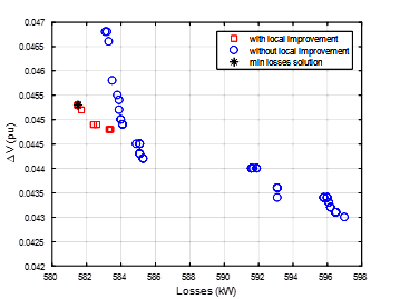
The Pareto’s front obtained with the best run of each variant (with local improvement and without local improvement) of the presented optimization algorithm are shown in Fig. 1, where is also shown the point that represents the referred best solution for minimum losses of 280.18 kW and maximum voltage deviation of 0.0411 pu.
Table 1 Optimization of the circuit of 136 nodes with fixed demand
| with local improvement | without local improvement | |||||
| Best | Mean | Worst | Best | Mean | Worst | |
| Losses(kW) | 280.18 | 280.19 | 280.21 | 280.21 | 280.46 | 281.28 |
| ΔVmax(pu) | 0.033 | 0.033 | 0.033 | 0.033 | 0.033 | 0.033 |
| Iterations | 12.0 | 17.2 | 27.0 | 70.0 | 106.1 | 126 |
| Time (s) | 23.8 | 30.4 | 42.3 | 4.1 | 5.6 | 6.4 |
Source: The authors.
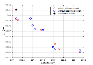
As can be seen (Fig. 1), the two objective functions are conflicting objectives. The solutions with lower losses present higher voltage deviations, while the solutions with lesser voltage deviations present higher losses.
Other solution that is near the point of the minimum losses solution but with better voltage is the solution marked in the frontier of solutions with local improvement. This solution with losses 280.21 kW and with voltage deviation 0.03945 pu (Vmin = 0.960551 pu), consists in the opening of branches: 7, 51, 53, 84, 90, 96, 106, 118, 126, 128, 137, 138, 139, 141, 144, 145, 147, 148, 150, 151, 156.
4.2. Solutions for the circuit of 136 nodes with variable demand
Souza [15] and Possagnolo [29] have determined the solution for minimum cost of daily losses of this example. That solution consists in the opening of the branches 7, 38, 51, 54, 84, 90, 96, 106, 118, 126, 135, 137, 138, 141, 144, 145, 147, 148, 150, 151, 155. This configuration have losses cost of $256.88, energy losses of 2211.285 kW.h and minimum voltage of 0.963865 pu (ΔVmax = 0.0361 pu).
The Table 2 shows the performance of both variants of the algorithm in ten runs of the optimization of the circuit of 136 nodes with variable demand. Again, the optimization with local improvement is better respect to the quality of solutions in both objective functions. All runs with local improvement are capable of obtaining the solutions with minimum values of the two objective functions.
Table 2 Optimization of the circuit of 136 nodes with variable demand
| with local improvement | without local improvement | |||||
| best | mean | worst | best | mean | worst | |
| Cost ($) | 256.88 | 256.88 | 256.88 | 256.88 | 256.94 | 257.08 |
| ΔVmax (pu) | 0.029 | 0.029 | 0.029 | 0.029 | 0.0305 | 0.0316 |
| Iterations | 11.0 | 16.1 | 24.0 | 81.0 | 111.6 | 194.0 |
| Time (s) | 96.3 | 126.3 | 172.3 | 15.4 | 20.4 | 35.5 |
Source: The authors.
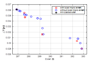
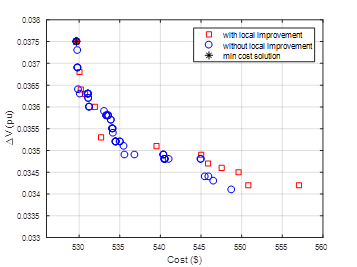
The Pareto’s front obtained with the best run of each variant of the optimization algorithm are shown in Fig. 2. In addition, the point with the best solution for the minimum cost presented in literature, is also shown.
4.3. Solutions for the circuit of 415 nodes with fixed demand
The circuit of 415 nodes have 473 branches and operates with 59 open branches. The reconfiguration of this circuit is a much more complex problem than the reconfiguration of the circuit of 136 nodes. In the following examples, a population of 60 solutions is used for the optimization without local improvement and a population of only 15 solutions is used for the optimization with local improvement.
The best solution for minimum losses of this example, slightly better than that found by Souza [14], have been presented by Possagnolo [29]. That solution with 581.55 kW of losses and minimum voltage of 0.95466 pu (ΔVmax = 0.04534 pu), consists in the opening of branches: 5, 13, 15, 16, 21, 26, 31, 54, 57, 59, 60, 73, 86, 87, 94, 96, 97, 111, 115, 136, 142, 149, 150, 155, 156, 158, 163, 168, 169, 178, 179, 191, 195, 199, 209, 214, 254, 256, 270, 294, 317, 322, 325, 354, 362, 369, 392, 395, 403, 404, 416, 423, 426, 431, 436, 437, 446, 449, 466.
The performance of both variants of the algorithm in the optimization of the circuit of 415 nodes with fixed demand is shown in Table 3.
Table 3 Optimization of the circuit of 415 nodes with fixed demand
| with local improvement | without local improvement | |||||
| best | mean | worst | best | mean | worst | |
| Losses (kW) | 581.55 | 581.68 | 582.61 | 583.13 | 583.80 | 585.92 |
| ΔVmax (pu) | 0.0432 | 0.0442 | 0.045 | 0.0429 | 0.0436 | 0.0452 |
| Iterations | 15.0 | 35.3 | 55.0 | 945.0 | 1701.2 | 2254.0 |
| Time (s) | 487.3 | 993.0 | 1491.6 | 499.5 | 885.0 | 1156.9 |
Source: The authors.
In this case, the optimization without local improvement is not capable of obtaining the solution of minimum losses in none of the ten runs. Besides, the mean value of minimum losses obtained with the optimization without local improvement is 0.36% worst than the obtained with local improvement. Also, the spread of the minimum losses obtained without local improvement is 2.79 kW, almost three times the spread of the solutions obtained with local improvement.
With respect to the second objective, the maximum voltage deviation obtained by the optimization without local improvement is 0.06% better than the obtained by the optimization with local improvement. Both variants of the algorithm are approximately the same respect to the calculation time.
The Pareto’s fronts for this case, obtained from the best run of each variant of the presented optimization algorithm, are shown in Fig. 3. In addition, is also shown the point of the best solution for minimum losses present in literature.
As can be seen (Fig. 3), the front of solutions obtained without local improvement is clearly separated from the zone of the minimum losses solution. Besides, the solutions with lower losses obtained without local improvement, have higher voltage deviations than the solutions obtained with local improvement.
4.4. Solutions for the circuit of 415 nodes with variable demand
The best solution for minimum losses cost for this example have been presented by Souza [15] and Possagnolo [29]. That solution with daily cost of $529.66 and minimum voltage of 0.962472 pu (ΔVmax = 0.03748 pu), consists in the opening of branches: 1, 2, 13, 15, 16, 26, 31, 40, 41, 50, 59, 73, 82, 94, 96, 97, 111, 115, 136, 146, 150, 155, 156, 158, 163, 168, 169, 178, 179, 190, 191, 194, 195, 209, 230, 254, 256, 267, 270, 294, 310, 321, 354, 362, 385, 389, 392, 395, 403, 404, 423, 424, 426, 436, 437, 439, 446, 449, 466.
Table 4 Optimization of the circuit of 415 nodes with variable demand
| with local improvement | without local improvement | |||||
| best | mean | worst | best | mean | worst | |
| Cost ($) | 529.66 | 530.00 | 530.49 | 529.70 | 530.03 | 531.31 |
| ΔVmax(pu) | 0.0342 | 0.0350 | 0.0360 | 0.0340 | 0.0343 | 0.0345 |
| Iterations | 17.0 | 41.6 | 69.0 | 1203.0 | 1700.0 | 2459.0 |
| Time (s) | 2148.1 | 4665.6 | 7537.6 | 2059.4 | 2896.8 | 4186.4 |
Source: The authors.
The performance of both variants of the algorithm in the optimization of the circuit of 415 nodes with variable demand is shown in Table 4. With respect to the first objective function, the mean value of minimum losses obtained with both variants of the algorithm is almost the same. However, the spread of the minimum losses obtained without local improvement is 1.61 kW, about twice the spread of the solutions obtained with local improvement. With respect to the second objective, the maximum voltage deviation obtained by the optimization without local improvement is 0.08% better than the obtained by the optimization with local improvement. In this case, the calculation time of the optimization without local improvement is about the 62% with respect to the optimization with local improvement.
The solutions of Pareto’s front obtained with the best run of each variant of the presented optimization algorithm are shown in Fig. 4. Again, the point of the best solution for minimum cost present in literature is shown for comparison.
As can be seen (Fig.4), this is the example in which both Pareto’s fronts are more similar between them. Other remarkable solution that is near in losses to the minimum losses solution but with better voltage is the solution marked in the frontier obtained without local improvement. This solution with losses cost of $529.9 and voltage deviation 0.03644 pu (Vmin = 0.963560 pu), consists in the opening of branches: 1, 2, 13, 15, 16, 26, 31, 40, 41, 50, 59, 73, 82, 94, 96, 97, 111, 115, 136, 142, 150, 155, 156, 158, 163, 168, 169, 178, 179, 190, 191, 194, 195, 221, 230, 254, 256, 266, 267, 282, 314, 321, 354, 362, 385, 389, 392, 395, 403, 404, 423, 424, 426, 436, 437, 439, 446, 449, 466.
Conclusion
In this work, the local improvement step commonly used in single-objective optimization is included in the multi-objective optimization by selecting at random the objective function that will be improved on each individual of the genetic algorithm population. That improvement is applied once the individual is produced by crossover or mutation.
Both variants of the algorithm, with or without local improvement, are capable to determine the frontier of Pareto for the multi-objective reconfiguration of distribution systems. However, the optimization with local improvement converges normally in lesser number of iterations to better non-dominated solutions. Besides, the use of the local improvement step reduce the spread among the solutions of consecutive runs, increasing the stability of results.
With respect to the calculation time, the optimization with local improvement employs more time per iteration and converge in less iterations. To reduce the calculation time, a much-reduced population of about 0.25-0.5 times the number of open branches of the circuit is used. However, even with this reduced population, in general the optimization with local improvement uses more calculation time in all cases.

