


 Inglés (pdf)
 Articulo en XML
 Referencias del artículo
 Enviar articulo por email
 Citado por SciELO
  Citado por Google
  Similares en
SciELO
Similares en
SciELO  Similares en Google
 Permalink
INTRODUCTION
Sulfonamides are a group of synthetic organic compounds that have played an important role as effective chemotherapeutics in bacterial and protozoal infections in veterinary medicine. Indications for sulfonamides are wide against both Gram negative and Gram-positive bacteria, owing to their wide spectrum of activity. Sulfonamides are used to treat infectious diseases of the digestive and respiratory tracts, secondary infections, mastitis, metritis, and foot rot [1-3]. All drugs of the sulfonamide group are currently included in Council Regulation (EEC) N.°2377/90 of 26 June 1990 laying down a community procedure for the establishment of maximum residue limits of veterinary medicinal products in foodstuffs of animal origin [4]. So, the existing EU Maximum Residue Levels (MRLs) for all drugs of the sulfonamide group is 100 µg/kg in all food-producing species [5].
Sulfadiazine (SD, 4-amino-N-2-pyrimidinylbenzenesulphonamide, molar mass 250.28 g.mol-1, CAS number 68-35-9, molecular structure shown in figure 1) is a sulfonamide drug employed sometimes in human and veterinarian therapeutics because it exhibits a wide spectrum against most gram-positive and gram-negative organisms [6-9]. It inhibits the multiplication of bacteria by acting as a competitive inhibitor of p-aminobenzoic acid in the folic acid metabolism cycle [1,10-12]. In spite of its continuous therapeutical use its equilibrium solubility data in aqueous-cosolvent mixtures is not yet complete [13].
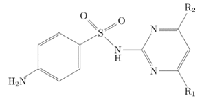
Sulfamethazine, (SMT, N1-(4,6-dimethyl-2-pyrimidinyl) sulfanilamide, figure 1), is broadly used in veterinary medicine to treat infectious diseases. SMT abuse in veterinary practice may lead to the presence of SMT residues in food; these residues are harmful to consumers because of their carcinogenic potential and risk of developing antibiotic resistance [14-16].
Sulfamethazine: R1 and R2 = CH3.
SMT has a low aqueous solubility, so solubility studies of this therapeutic agent are important. And within research related to solubility, co-solvency is perhaps the most relevant strategy to increase the solubility of a drug.
The other hand, that predictive methods of physicochemical properties of drugs, in particular those intended for estimating their solubilities in neat solvents and in solvent mixtures, are very important for pharmaceutical and chemical industries [17]. This is because these calculating methods could allow the optimization of several design and development processes. Thus, two of the most widely used methods for predicting solubility in co-solvent mixtures are the Yalkowsky-Roseman (YR) [18,19] model and extended Hildebrand solubility approach (EHSA) [20-23].
This work presents a physicochemical study about the solubility prediction of SD and SMT in binary mixtures conformed by ethylene glycol + water. The study was done based on the Yalkowsky-Roseman (YR) model and extended Hildebrand solubility approach (EHSA) by using experimental solubility values and some properties relative to the fusion of this drug [24], evaluating the relevance of these models, in predicting the solubility of SD and SMR in the ethylene glycol + water cosolvent system, at different temperatures, to strengthen the data bases, related to the solubility of these drugs, providing a tool that offers reliable information, for the development of processes that involve these drugs and the solvents used.
THEORETICAL
Yalkowsky-Roseman model
The logarithmic solubilities of Yalkowsky-Roseman (YR) model for a solute in the different solvent mixtures including neat solvents were determined with the help of equation [18,25,26].

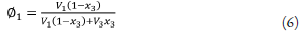
Where x 3,1+2 is the drug solubility calculated in the cosolvent mixture considered, x 3,1 is the drug solubility in the neat cosolvent, x 3,2 is the drug solubility in neat water, and f is the volume fraction of cosolvent in the mixed solvent. This last term is calculated assuming

where, V 1 and V 2 are the respective volumes of cosolvent and water.
The equation 1 can be written as [27]:

which suggests a linear relationship between ln x 3,1+2 and solvent composition [27]. This exponential increase in solubility with cosolvent composition has been repeatedly observed in the literature [27].
Extended Hildebrand Solubility Approach
The extended Hildebrand solubility approach (EHSA), a modification of the Hilde-brand-Scatchard equation, permits calculation of the solubility of polar and non-polar solutes in solvents ranging from non-polar hydrocarbons to highly polar solvents such as water, ethanol, and glycols [28]. The solubility parameters of solute and solvent were introduced to explain the behavior of regular and irregular solutions [29,30]. The extended Hildebrand solubility approach has been developed to reproduce the solubility of drugs and other solids in the binary solvent systems [31-33].
Solubility on the mole fraction scale, x3, may be represented by the equation:

where x3 id is the ideal solubility of the crystalline solid, and y3 is the solute activity coefficient in mole fraction terms. Scatchard [34] and Hildebrand and Scott [35] formulated the solubility equation for regular solutions:
 where
where
V 3 is the molar volume of the hypothetical supercooled liquid solute (subscript 3), ϕ 1 is the volume fraction of the solvent (subscript l), R is the molar gas constant, and T is the absolute temperature of the experiment.
The terms e 11 and e22 are the cohesive energy densities of solvent and solute, and e 12 is expressed in regular solution theory as a geometric mean of the solvent and solute cohesive energy densities and is expressed as W in this work [30,36,37]:

The square roots of the cohesive energy densities of solute and solvent, called solubility parameters and given the symbol, are obtained for the solvent from the energy or heat of vaporization per volume:
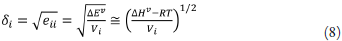
Replacing e ii with , in equation 5, the expression becomes:

replacing the first term by, and factoring the second one:

Martha Sofía Vargas-Santana, Ana María Cruz-González, Nestor Enrique Cerquera et al.
Substituting equation 10 into equation 4, one obtains the Hildebrand-Scatchard solubility equation [38]:

where

Where ∆H fus is the molar enthalpy of fusion of the pure solute (at the melting point), Tfus is the absolute melting point, Tis the absolute solution temperature, R is the constant gas (8.314j·mol-1·K-1) and ∆C p is the difference between the molar heat capacity of the crystalline form and the molar heat capacity of the hypothetical supercooled liquid form, both at the solution temperature. Since ∆C P , values are not commonly reported, they may be approximated to the entropy of fusion, ∆S fus calculated as follows:

replacing δ 1 δ 3 by W, equation 9 becomes

So, equation 4 is rewritten as [39,40]

Here, the term is equal to (where, is the Walker parameter). The factor can be calculated from experimental data by means of [41,42]:
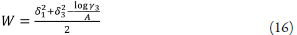
The experimental values of the W parameter can be correlated by means of regression analysis by using regular polynomials as a function of δ 1 as follows [36,43]:

These empiric models can be used to estimate the drug solubility by means of back-calculation, resolving this property from the specific value obtained in the respective polynomial regression [38,44].
RESULTS AND DISCUSSION
The experimental solubility data of SD and SMT in (EG + W) cosolvent mixtures were taken from Cruz et al. [ 6] and Adi et al. [ 24]. Table 1 presents basic information for the development of the YR and EHSA models.
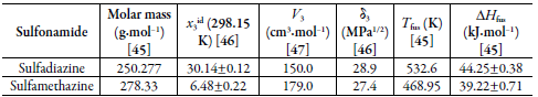
The volumetric behavior and polarity of (EG+ W) mixtures, as a function of the com-position, are shown in table 2. Volume fractions and Hildebrand solubility parameters were calculated assuming additive behavior.
Table 2 Some physicochemical properties of pure solvents and (EG + W) cosolvent mixtures (298.15 K).
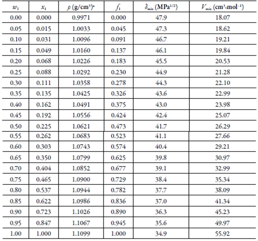
a The density was calculated by regression, from the density data published by Egorov et al. [ 48].
Tables 3 and 4 presents the solubility data of the SD and SMT calculated using the YR model, and standard deviations (SD) with respect to the experimental values.
Table 3 Calculated solubility of SD in {ethylene glycol (1) + water (2)} mixtures by using the equations 3, and standard deviations with respect to the experimental values.
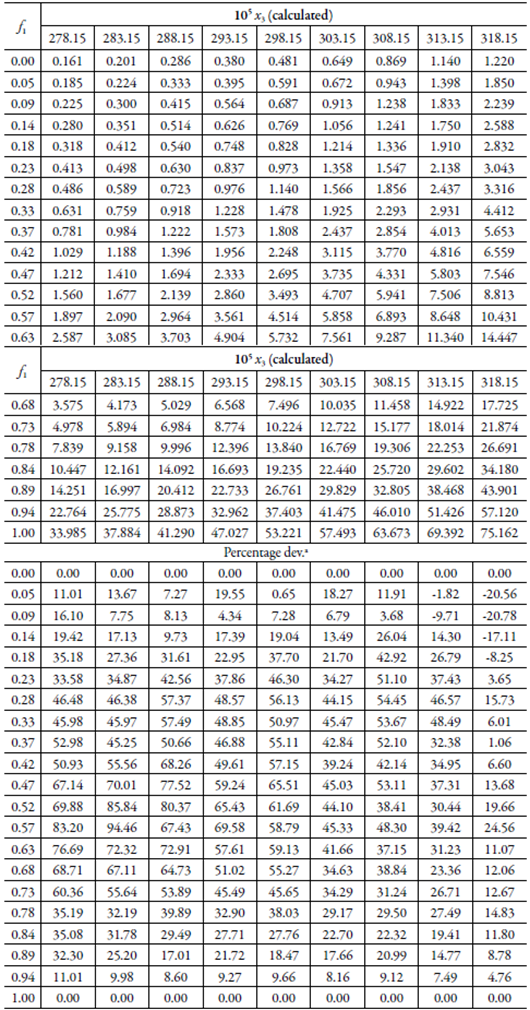
a Calculated as 100|x3cal- x3exp|/| x3exp|
Table 4 Calculated solubility of SMT in {ethylene glycol (1) + water (2)} mixtures by using the equations 3, and standard deviations with respect to the experimental values.
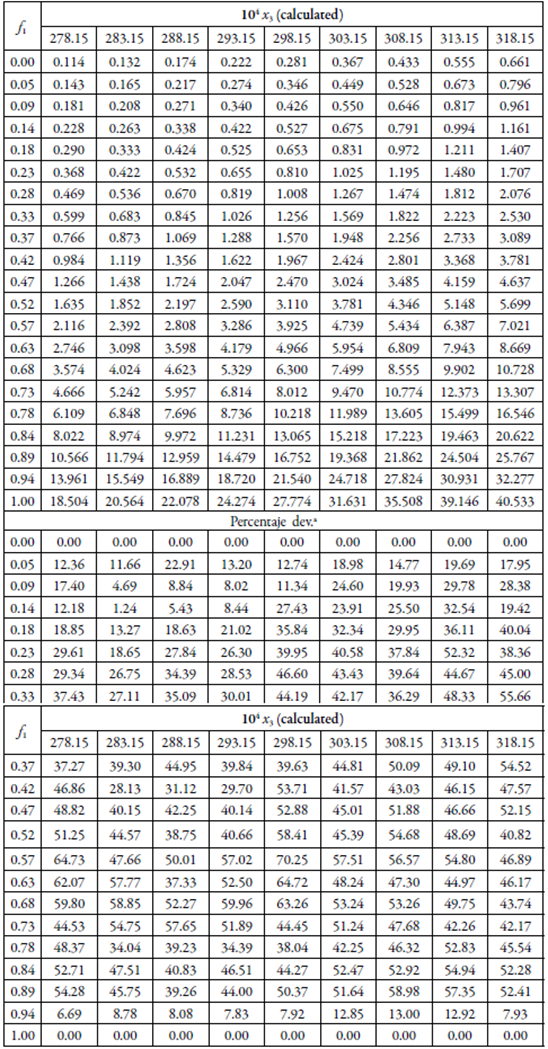
aCalculated as 100|x3 cal- x3 exp|/| x3 exp|
When evaluating the individual deviations of the calculated data with respect to the experimental data, relatively large deviations are observed, with a maximum of 94.46% for the SD and 57.51% for the SMT. As a general measure of the validity of the two models, the mean percentage deviation values were calculated according to equation 18, where is the number of points of the resulting cosolvent composition.
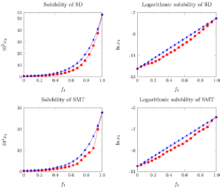
Thus, in general, the YR model presents an MPD of 31.1% for SD and 34.8% for SMT, an acceptable percentage for the pharmaceutical industry. Figure 2 shows that, in general, the deviations were greater in intermediate mixtures and are reduced in mixtures rich in either of the two solvents.
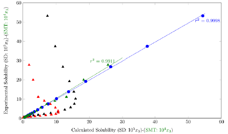
On the other hand, when plotting the calculated solubility vs. the experimental solubility (figure 3), pooled data is obtained, indicating a good predictability of the model.
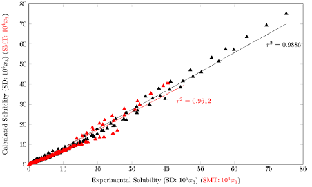
Figure 3 Calculated solubility vs. experimental solubility by YR model of SD and SMT in (EG + W) mixtures.
Figure 4 shows the experimental solubility of SD and SMT in (EG + W) mixtures, the solubility calculated using the equation for regular solutions, and the solubility calculated using the MESH as a function of the solubility parameter of solvent mixtures; the logarithm of experimental solubility and calculated solubility by EHSA are also presented. The experimental solubility is greater than the calculated solubility by using the regular solution model in every one of the mixtures evaluated. This result could be attributed to the fact that this semiempirical model does not consider specific interactions between solvent and solute, and all the involved compounds present polar groups that could interact by hydrogen bonding. In principle, SD and SMT would behave like a Lewis base in mixtures rich in water due to the pair of free electrons of its groups -SO2-, -NH2- and =N- in addition to the fact that water is more acidic than EG according to the acid and basicity parameters of Kamlet-Taft (α 2 = 1.017±0.0236, α 1 = 0.792±0.004 [49], and β 2 = 0.14 β1=0.51 [50]), and as a Lewis acid in intermediate and rich mixtures in EG due to the hydrogen of its groups -NH2- and -NH-. Although, it is evident that the Hildebrand model of regular solutions does not allow obtaining data consistent with the experimental ones, the results obtained with the EHSA model, using the W calculated with the second order polynomial, overlap with the experimental data.
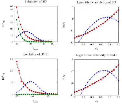
Figure 4 Experimental and calculated solubility of SD and SMT at 298.15 K (A: Calculated solubility by EHSA model (Polynomial 2); ●: experimental solubility; ●: Calculated solubility by EHSA model (Polynomial 1) and ●: Calculated solubility by regular solution model.
Regarding the solubility calculated using the EHSA model, to calculate the parameter (table 5), the calculated 3 m¡x value was used (table 2). On the other hand, the parameter A, is presented in table 5 too. Figure 5 shows that the variation of the parameter with respect to the solubility parameter of solvent mixtures, presents deviation from linear behavior.
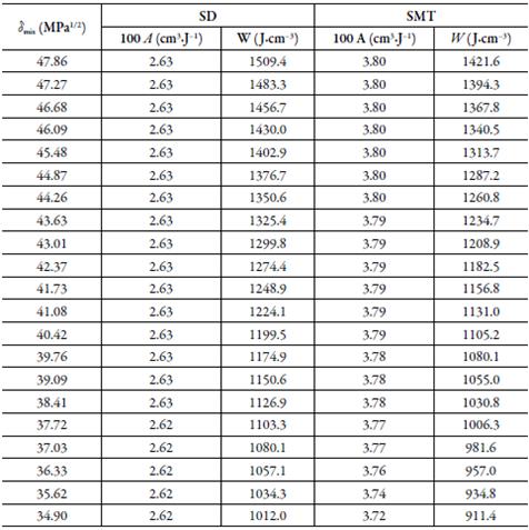
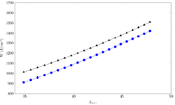
Figure 5 W parameter as a function of the solubility parameter of the solvent mixtures in (EG + W) mixtures (SD: ●; SMT: ●).
W values were adjusted to regular polynomials in orders from 2 to 5 (equation 17). Nevertheless, linear model was also evaluated with comparative purposes. Table 6 and table 7, summarizes the coefficients obtained in all the regular polynomials from degrees one to five for SD an SMT.
Table 6 Coefficients and statistical parameters of regular polynomials in several orders of W as a function of solubility δ mix free of SD (equation 17) in (EG + water) mixtures.
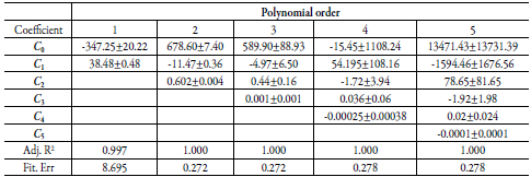
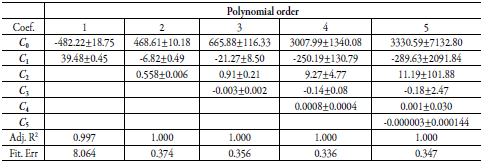
Table 7 Coefficients and statistical parameters of regular polynomials in several orders of W as a function of solubility δmix free of SMT (equation 17) in (EG + water) mixtures.
Tables 8 and 9 report the calculated solubility of SD and SMT and the respective percentages of deviation. When using the values of the factor W calculated with the polynomial of order 1, the deviations of the calculated data with respect to the experimental data is greater than 60%, indicating that the model is not the appropriate one. However, when using the results of W, calculated with a polynomial greater than or equal to 2, the deviations are low, presenting a good correlation between the calculated and experimental data.
Table 8 Calculated solubility of sulfadiazine in (EG + water) mixtures by using the W parameters obtained from regression models in orders 1, 2, 3, 4 and 5, and standard deviations with respect to the experimental values, at 298.15 K.
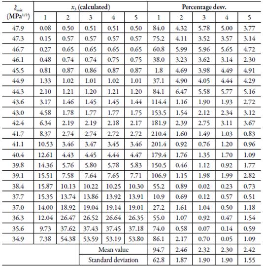
Table 9 Calculated solubility of sulfamethazine in EG + water mixtures by using the W parameters obtained from regression models in orders 1, 2, 3, 4 and 5, and standard deviations with respect to the experimental values, at 298.15 K.
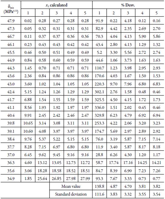
These results can be corroborated in figure 6, where the data calculated with polynomial 1 show a high dispersion, contrary to the data calculated with the polynomial of order 2, which present a correlation coefficient greater than 0.99.
CONCLUSIONS
The results obtained from the Yalkowsky-Roseman linear model do not present a good correlation with the experimental data, possibly due to the simplicity of the model, which does not consider the solute-solvent and solvent-solvent molecular interactions. However, the results of the extended Hildebrand solubility approach (EHSA), calculated with a polynomial greater than or equal to two, present interesting correlations, with deviation percentages less than 3%.

