Inglés (pdf)
 Articulo en XML
 Referencias del artículo
 Enviar articulo por email
 Citado por SciELO
  Citado por Google
  Similares en
SciELO
Similares en
SciELO  Similares en Google
 Permalink
1. Introduction
In this study we are concerned with the problem of approximating a locally unique solution x* of equation
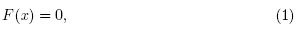
where  is a nonlinear function, D is a convex subset of S and S is
  or
or  . Newton-like methods are famous for finding solution of (1), these methods are usually studied based on: semi-local and local convergence. The semi-local convergence matter is, based on the information around an initial point, to give conditions ensuring the convergence of the iterative procedure; while the local one is, based on the information around a solution, to find estimates of the radii of convergence balls [3,5,20,21,22,24,26].
Third order methods such as Euler's, Halley's, super Halley's, Chebyshev's [2-28] require the evaluation of the second derivative F" at each step, which in general is very expensive. That is why many authors have used higher order multipoint methods [2-28Α. In this paper, we study the local convergence of third order Steffensen-type method defined for each n = 0,1, 2, ... by
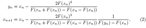
where x0 is an initial point. Method [2] was studied in [18] under hypotheses reaching upto the fourth derivative of function F.
Other single and multi-point methods can be found in [1,3,20,25] and the references therein. The local convergence of the preceding methods has been shown under hypotheses up to the fourth derivative (or even higher). These hypotheses restrict the applicability of these methods. As a motivational example, let us define function f on D =  by
by
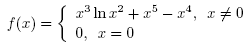
Choose x* = 1. We have that
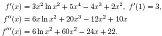
Then, obviously, function f''' is unbounded on D. In the present paper we only use hypotheses on the first Frechet derivative. This way we expand the applicability of method (2).
The rest of the paper is organized as follows: Section 2 contains the local convergence analysis of methods (2). The numerical examples are presented in the concluding Section 3.
2. Local convergence
We present the local convergence analysis of method (2) in this section. Let  stand for the open and closed balls in S, respectively, with center
  and of radius p > 0.
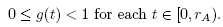
Let L0 > 0, L > 0, M0 > 0, M > 0 and α > 0 be given parameters. It is convenient for the local convergence analysis of method(2) that follows to define some functions and parameters. Define function on the interval 
By
and parameters

Notice that if:
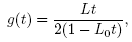
We have that g(rA) = 0, and
Define function g1 on the interval  by
by
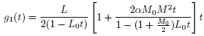
and set
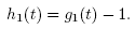
We get that . It follows from the Intermediate Value Theorem that function h1 has zeros in the interval (0,r0). Denote by r
1 the smallest such zero. Moreover, define function on the interval
. It follows from the Intermediate Value Theorem that function h1 has zeros in the interval (0,r0). Denote by r
1 the smallest such zero. Moreover, define function on the interval  by
by
and set
Then, we have that  and
and  . Hence, function h has a smallest zero rp
 . Furthermore, define function on the interval
  by
by
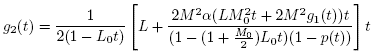
and set
Then, we have  and
and  Hence, function h
2
has a smallest zero denoted by r
2
. Set
Hence, function h
2
has a smallest zero denoted by r
2
. Set

Then, we get that for each 


And

Next, using the above notation we present the local convergence analysis of method (2).
Theorem 2.1. Let F :  be a differentiable function. Suppose that there exist
 and M > 0 such that for each x, y Є
D
the following hold
and M > 0 such that for each x, y Є
D
the following hold


and

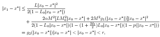
where r is defined by (3). Then, the sequence generated by method (2) for
 is well defined, remains in
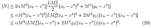
 for each n = 0,1, 2, … and converges to x*. Moreover, the following estimates hold for each n = 0,1, 2, …,

And

where the "g" functions are defined above Theorem 2.1. Furthermore, if that there exists such that
 , then the limit point x* is the only solution of equation F(x) = 0 in
  .
.
Proof. We shall use induction to show estimates (13) and (14). Using the hypothesis 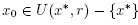 , the definition of r and (8) we get that

It follows from (15) and the Banach Lemma on invertible functions [3,5,19,20,22,23] that F'(x0) is invertible and

We can write by (7) that

Then, we have by (10), (11) and (17) that
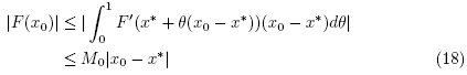
and
where we used  for each
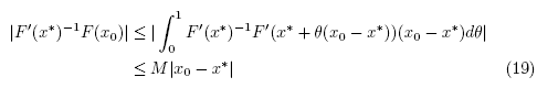
 . We also have by (18) and (12) that
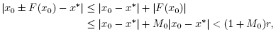
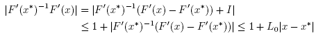
so . Next we shall show that
  is invertible. Using the definition of r0, (8) and (18), we get in turn that
It follows from (20) that  is invertible and
Hence, y0 is well defined by the first substep of method (2) for n = 0. Then, we can write
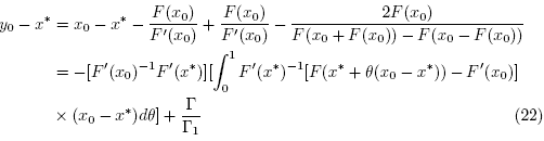
where 
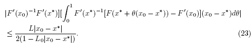
 The first expression at the right hand side of (22), using (9) and (16) gives
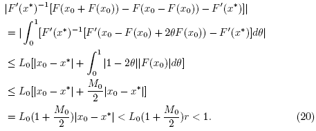
Using (7), (9), (18) and (19) the numerator of the second expression in (22) gives
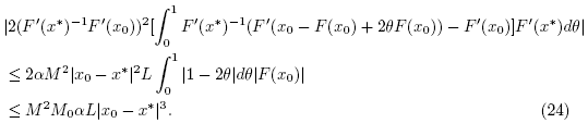
Then, it follows from (4), (16), (21), (22)-(24) that
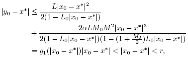
which shows (13) for n = 0 and . Next, we shall show that F(x
0
) - F(y
0
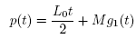
) is invertible. Using the definition of function p, x0 ≠ x*, (5), (8), (13) (for n = 0), we get in turn that
. Next, we shall show that F(x
0
) - F(y
0
) is invertible. Using the definition of function p, x0 ≠ x*, (5), (8), (13) (for n = 0), we get in turn that
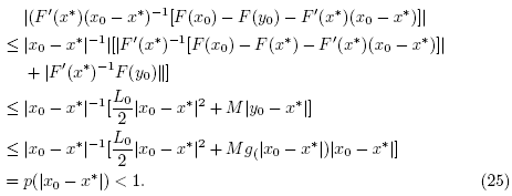
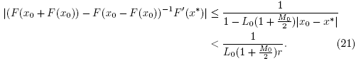
It follows from (25) that F(x0) -F(y0) is invertible and
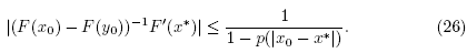
Hence, x1 is well defined by the second step of method (2) for n = 0. We can also write that
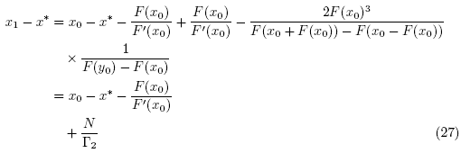
Where

and 
Then, using (6), (16), (21), (23) and (26)-(29), we get that
which shows (14) for n = 0 and  . By simply replacing x0,y0,x1 by xk, yk, xk+1 in the preceding estimates we arrive at estimates (13) and (14). Using the estimate
  we deduce that
 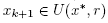 and
and 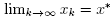 .
.
To show the uniqueness part, let 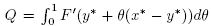 for some y* €
  with F(y*) = 0. Using (7) we get that
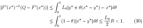
It follows from (30) and the Banach Lemma on invertible functions that Q is invertible. Finally, from the identity 0 = F(x*) - F(y*) = Q(x* - y*) , we conclude that x* = y*.
Remark 2.2. (1) In view of (9) and the estimate
condition (11) can be dropped and M can be replaced by
(2) The results obtained here can be used for operators F satisfying autonomous differential equations [3] of the form
where P is a continuous operator. Then, since F'(x*) = P(F(x*)) = P(0), we can apply the results without actually knowing x* . For example, let F(x) = ex - 1. Then, we can choose: P(x) = x + 1.
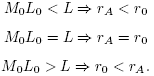
(3) The radius r A was shown by us to be the convergence radius of Newton's method [1-5]

under the conditions (9) and (10). It follows from the definition of r that the convergence radius r of the method (2) cannot be larger than the convergence radius of the second order Newton's method (31) if L 0 M 0 ≥ L. Even in the case L 0 M 0 < L, still r may be smaller than r A .
As already noted in [3,5] is at least as large as the convergence ball given by Rheinboldt [25]
In particular, for L 0 < L we have that

and
That is our convergence ball r A is at most three times larger than Rhein-boldt's. The same value for r R was given by Traub (26).
(4) It is worth noticing that method (2) is not changing when we use the conditions of Theorem 2.1 instead of the stronger conditions used in [2,4,9-28]. Moreover, we can compute the computational order of convergence (COC) defined by
or the approximate computational order of convergence
This way we obtain in practice the order of convergence in a way that avoids the bounds involving estimates using estimates higher than the first Frechet derivative of operator F.
3. Numerical Examples
We present numerical examples in this section.
Example 3.1. Let D = . Define function f of D by

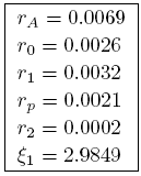
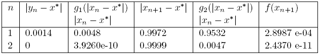
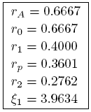
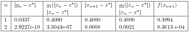
Then we have for x* =0 that L0 = L = M = M0 = 1, α =1. The parameters are given in Table 1 and error estimates are given in Table 2.
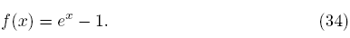
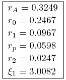
Using (34) and x* = 0, we get that L 0 = e - 1 <L = M = M0 = e,α =1. The parameters are given in Table 3 and error estimates are given in Table 4.
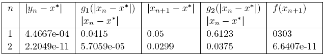
Example 3.3. Returning back to the motivational example at the introduction of this study, we have L 0 = L = 96.662907, M = 2, M0 = 3M, α = 1. The parameters are given in Table 5 and error estimates are given in Table 6.