


 Inglés (pdf)
 Articulo en XML
 Referencias del artículo
 Enviar articulo por email
 Citado por SciELO
  Citado por Google
  Similares en
SciELO
Similares en
SciELO  Similares en Google
 Permalink
1. Introduction
From a standard advection-dispersion equation, new problems arise by considering fractional time and/or space derivatives. Furthermore, for the new problems it makes sense to consider inverse problems of different types. These mathematical problems have applications in physics, chemistry, biology and several branches of engineering, among others (see [4,14,15,16,17]). Fractional advection-dispersion equations and the inverse problems based on them are specially valuable in groundwater hydrology and other instances of transport in porous media [3,5].
The main features of the present work are:
(1) An inverse problem based on a time fractional advection-dispersion equation is solved.
(2) The equation is one-dimensional and the evolution takes place in a semi-infinite setting. As a first approximation, this is not a drawback, according to Benson et al. in [3]. They state: A typical question that a contaminant hydrogeologist wishes to answer is How far and how fast will a tracer move? As a first approximation, this reduces most problems to one spatial dimension.
(3) The fractional derivative is a Caputo fractional derivative.
(4) The inverse problem is severely ill-posed.
(5) Discrete mollification is the chosen regularization tool.
Several inverse problems based on time fractional differential equations have been successfully solved by discrete mollification [12,13] but to the best of our knowledge, this is the first time that this regularization method is implemented for the stable solution of a time fractional inverse advection-dispersion equation (TFIADP).
The precise statement of the mathematical problem is introduced in the next section. At a first glance, it is similar to the problems in [14] and several papers by Zheng and Wei [15,16,17]. These publications are the main precedents of this paper and the crucial difference between all of them and our work, is the use of discrete mollification as regularization procedure.
The rest of the paper is organized as follows: As mentioned before, section 2 introduces the mathematical setting. It includes the relevant equations, the ill-posedness of the inverse problem and a short introduction to discrete mollification. Sections 3 and 4 deal with the space marching numerical scheme and they include the proofs of the main results. The numerical examples are in section 5 and the last section is dedicated to some final remarks.
2. Mathematical setting
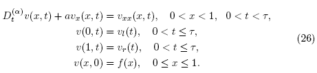
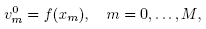
Whenever an inverse problem is introduced, there is a direct problem in which it is based. In our case is the following:
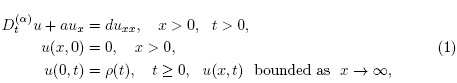
where u is the solute concentration, u
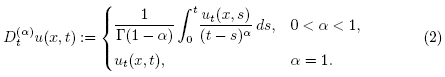
x is the dispersion flux, the constants a > 0, d > 0 represent the average fluid velocity and the dispersion coefficient, respectively, and  denotes the Caputo fractional derivative of order α,
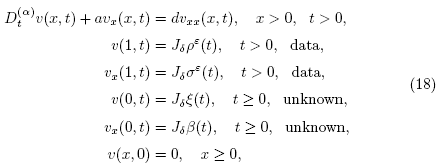
We are interested in the following time fractional inverse advection-dispersion problem (TFIADP):
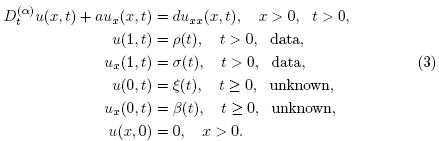
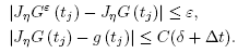
The distributed interior data functions p and σ are not known exactly. Moreover, their measured approximations  and
and  satisfy the estimates
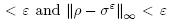 for a prescribed maximum level of noise in the data
We are interested in a numerical identification process of  and β based on the overdetermined interior data and . They are measurements on the direct problem evolving process. Our scope is the numerical solution of the inverse problem by discrete mollification, and we do not address theoretical issues related to existence, uniqueness and identifiability of the solute concentration u or the flux of solute ux.
2.1. The discrete mollification operator
The discrete mollification method [9,2] is based on replacing a discrete set of data  which may consist of evaluations or cell averages of a real function y = y(t) at equidistant grid points
  by its mollified version
  , where
  is the discrete mollification operator defined
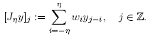
Here, the support parameter  indicates the width of the mollification stencil, and the weights w
i
satisfy
indicates the width of the mollification stencil, and the weights w
i
satisfy  and
and  along with
  The weights w¿ are defined as follows:
Let  and p > 0. We choose n as the unique non-negative integer such that

Actually
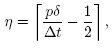
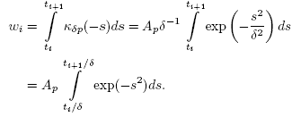
where  means the ceiling function. The weights are obtained by numerical integration of the truncated Gaussian kernel
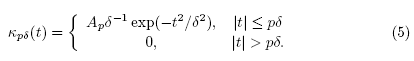
where the normalization constant
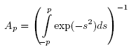
is chosen in such a way that  Based on this kernel, the mollification weights are computed by
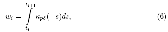
where

We usually take p = 3 and refer to δ as the mollification parameter, whose role is to determine the shape of the truncated Gaussian kernel.
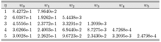
Chosen in this way, the mollification weights w j 's are independent of Δt, namely,
Recall that
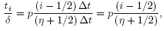
then the wi's depend only on p, 5 and n. Some weights are shown in Table 1.
Remark 2.1. Discrete mollification is a convolution operator and as such, it requires n values to the right and to the left of any given point. Suppose the function g(t) is defined in I = [0,1]. Then, unless some extensions to the left of 0 and to the right of 1 are established, the only points at which discrete mollification can be computed are points of the interval I δ = [pδ,1 - pδ]. Some useful extensions of the data outside the interval are presented in [2]. However, in this paper, our estimates are given for the interior points of the interval I δ. All mollifications in this paper are with respect to the time variable, due to the fact that a space marching finite difference scheme is implemented.
Discrete mollification satisfies the following estimates (see [7] and [8]).
Theorem 2.2.
Let g be a sufficiently smooth real function bounded in
 . Let G be its discrete version defined on T, a uniform meshgrid with discretization parameter
  is other discrete function defined on T and satisfies
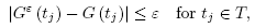
then there is a constant C > 0 independent of ô such that
Also,
2.2. Fractional derivatives and mollification
The presence of a derivative inside the integral in (2) is an indicator of the ill-conditioning of Caputo fractional derivatives when applied to noisy data. More precisely, if D
(α)
g is sought but we only have an approximation of g(t) denoted by  and satisfying
  instead of recovering D
(α)
g we look for a mollified approximation
instead of recovering D
(α)
g we look for a mollified approximation  . This approximation satisfies the following error estimate [13]:
Lemma 2.3. Let  g and
g and defined on I so that
 Additionally, suppose
 and both
 and g
e
are uniformly Lipschitz on I
δ
. Then there exists a constant C, independent of δ, such that
and g
e
are uniformly Lipschitz on I
δ
. Then there exists a constant C, independent of δ, such that
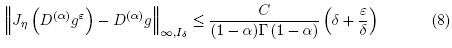
Remark 2.4. The right-hand side of (8) includes the factor  as a clear indication that computing the Caputo fractional derivative of a noisy approximation of the actual function, is an ill-posed problem. To obtain a formal convergence estimate, the parameters e and δ have to be linked in order for the right-hand side to tend to 0 as ε tends to ∞.
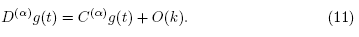
A discrete approximation of the Caputo fractional derivative can be obtained by a quadrature formula as described in [13]:
Lemma 2.5. Let g be a continuously differentiable function, and let k be a positive integer. Then the operator
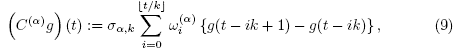
where denotes the floor function,

satisfies the first order approximation
2.3. Mollified problem
The inverse problem (3) is a severely ill-posed problem in the high frequency components as the following argument indicates. We assume that all the functions can be extended to the whole line -∞ < t < ∞ by defining them to be zero for t < 0, and that lie in L
2
( ) with respect to the variable t. Applying the Fourier transform with respect to t at
 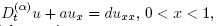 we obtain [6, p. 17] the second-order differential equation

where 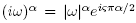 and
and  The general solution of (12) is given by

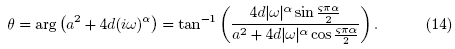
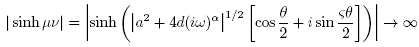
where k1 and k2 are the two square roots of the complex number  i.e.,
i.e.,
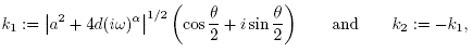
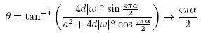
with
Setting 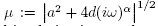 and
and  sin
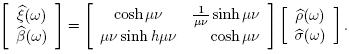
sin , the general solution (13) and its derivative can be rewritten in the form

When x = 0, it follows from expressions (15), using data from inverse problem (3), that
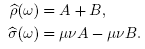
Solving this system for A and B, we get
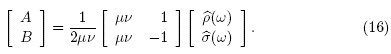
On the other hand, using the unknowns of the inverse problem (3) when x = 1, we get
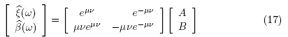
We derive from (16) and (17) that
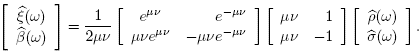
Thus,
Since

and
whenever  it follows that

and
whenever  and therefore solving the inverse problem (3), i.e., obtaining
  and β from p and σ, amplifies the error in a high-frequency component by the factor exp
 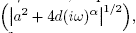 showing that the TFIADP is highly ill posed in the high-frequency components.
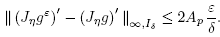
In the stabilized (mollified) problem,  and
and  satisfy
where 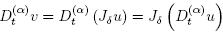 as stated in [10].
3. Mollified space marching finite difference scheme
Let  be a positive real number and let Δx = h and Δt = k be the parameters of the finite difference discretization. For each
  with
with  and each
  with
with  we denote by
  and
and  the computed approximations of the mollified solute concentration v(mh, nk), mollified flux of solute v
x
(mh, nk), and time fractional partial derivative of time partial derivative of mollified solute concentration
the computed approximations of the mollified solute concentration v(mh, nk), mollified flux of solute v
x
(mh, nk), and time fractional partial derivative of time partial derivative of mollified solute concentration 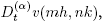 respectively. Following Murio [12], the space marching finite difference scheme proposed is given by the system
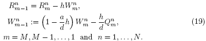
The values of  and
and 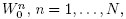 are the calculated approximations for the exact solute concentration
  and dispersion flux β(nk), respectively, at the grid points of the active boundary x = 0.
The next algorithm uses the finite differences scheme (19) to approximate the solution of the mollified problem (18). Notice that the evaluation of the time fractional derivative has to be performed in the indicated increasing order of values of time at each space grid position.
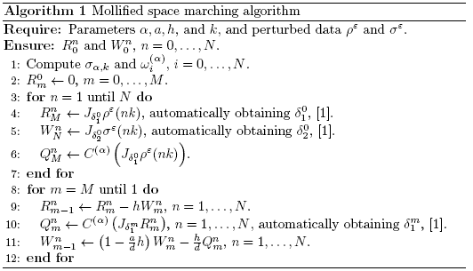
Remark 3.1. are obtained from the noisy data.
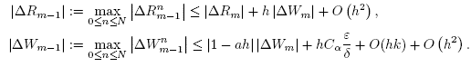
For error estimates, we introduce the discrete error functions

for each m Є {0,...,M}, and each n Є {0,..., N}. We also define

for each m Є { 0,....., M}.
Lemma 3.2. There exists a constant E > 0 such that

Proof. By Theorem (2.2), for each n Є {0,..., N}, there exist positive constants Cn y Dn such that

and

and consequently
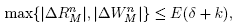
with E := max{Cn, Dn | n = 0,..., N}. By taking the maximum over n, the desired result is obtained. 
The next lemma shows the effect of the mollification in the discrete approximation of the Caputo fractional derivative.
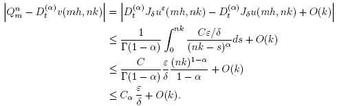
Lemma 3.3. There exists a constant Cα > 0 such that
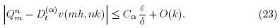
Proof. By lemma 2.5 and theorem 2.2,

Theorem 3.4 (formal convergence of the algorithm). The mollified space marching algorithm (1) converges to the solution of the inverse problem (3).
Proof. Without loss of generality, assume the dispersion coefficient d = 1. Expanding the mollified solute concentration v(x, t) by the Taylor series, we obtain
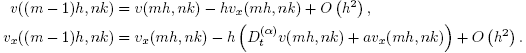
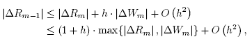
Hence the discrete errors (20) can be expressed as
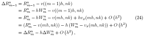
and
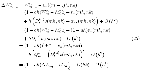
It follows from (24) and (25) that
and
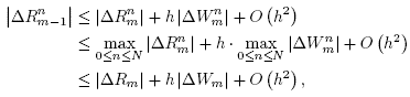
and therefore
Consequently
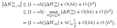
and
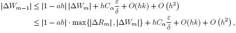
so that
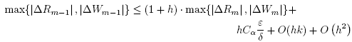
for m = M, M - 1,..., 1, and for any 0 < h < 1/a. It is readily verified by induction that
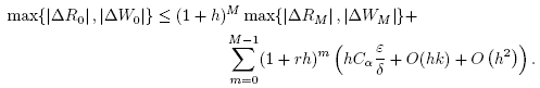
Hence
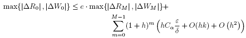
for all sufficiently small h > 0. Since
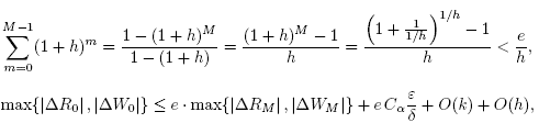
and by lemma 3.2 we obtain the estimate

for some constant C > 0. To ge(t convergence), the choice =  shows that max
 =
= , which implies formal convergence as ε, h and k → 0.
4. Data generation for TFIADP
In order to generate the necessary data for modeling the TFIADP, it is necessary to first solve the corresponding TFADP (the direct problem). Since a simple exact solution for the direct problem is not available, we implement an implicit finite difference scheme based on the scheme proposed by Murio [11], and then use the finite difference approximation as a reference solution, the closest we are from the exact solution.
The TFADP to solve is
The description of the scheme is as follows: Let M and N be positive integers and let  and
and  be the finite difference grid sizes. For each m Є {0,…, M}, and each n Є {0,…, N}, let
  be the computed approximations of
  , where xm = mh, and tn = nk are the grid point in the space interval [0,1] and time interval [0, t], respectively. We approximate the partial differential equation
 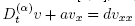 with the consistent finite-difference scheme
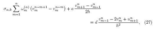
obtaining for internal nodes (m = 1 , 2,..., M - 1) and n = 1,
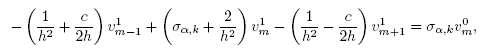
and for n = 2,...,N,
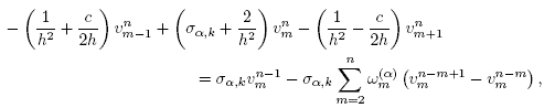
with boundary conditions
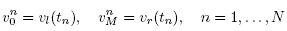
and initial condition
where  and
and  are given by (10).
The procedure to generate data for Algorithm 1 consists on using scheme (27) for obtaining approximate solutions of the direct problems
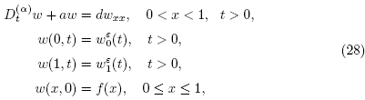
and
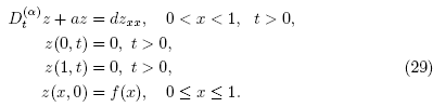
Setting v(x,t) := w(x,t) - z(x,t), data v(1,t) = w(1,t) - z(1,t) =  (t) and v
x
(1,t) = w
x
(1,t) - z
x
(1,t) are used to initialize Algorithm 1. In this way we obtain v(0,t) = w(0,t) - z(0,t) =
(t) and v
x
(1,t) = w
x
(1,t) - z
x
(1,t) are used to initialize Algorithm 1. In this way we obtain v(0,t) = w(0,t) - z(0,t) =  (t) and v
x
(0, t) = w
x
(0,t) - z
x
(0,t) as "exact solution" of the inverse problem (18). The derivatives v
x
(0,t
n
) and v
x
(1, t
n
) are computed by the forward difference schemes
(t) and v
x
(0, t) = w
x
(0,t) - z
x
(0,t) as "exact solution" of the inverse problem (18). The derivatives v
x
(0,t
n
) and v
x
(1, t
n
) are computed by the forward difference schemes
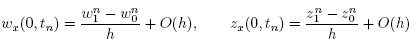
and

Perturbed approximations of the data for the TFIADP (18) at x =1 are simulated by adding random errors

where the ε n 's are random number uniformly distributed in [-ε, ε], and the magnitude ε indicates a noise relative level.
5. Numerical examples
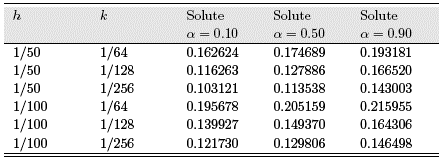
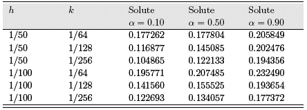
In order to test the stability and accuracy of the algorithm, we consider a selection of average noise perturbations, and space and time discretization parameters, h and k. The solute concentration and flux of solute errors at the boundary x = 0 are measured by the root mean square
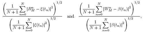
where the "exact" values u(0,nk) and u x (0,nk) are the computed (approximate) solutions for the solute concentration, and flux of solute of the direct problem, as explained in section 4.
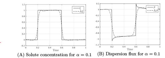
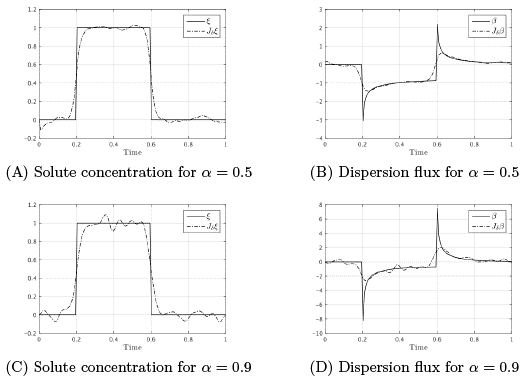
Example 5.1. This experiment consists on the recovery of a unit step boundary distribution of solute concentration at x = 0 from interior data measurements at x = 1.
We solve the TFADP's (28) and (29) using (27) with boundary conditions
w 1(t) = 0, and time fractional orders α = 0.10,0.50,0.90, grid sizes h = 0.01, k = 1/128 and noise level ε = 0.05. The numerical results for mollified solute concentration v and dispersion flux v x , after applying the mollified space marching algorithm (1) are shown in Figures (1) and (2).
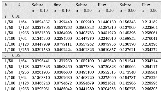
Numerical results for parameters h = 1/50,1/100 and k = 1/64,1/128,1/256, and noise levels ε = 0.01, 0.05 are listed in Tables (2) and (3). The relative errors for the reconstructed dispersion fluxes are not shown due to the singularities present in the exact dispersion flux solution functions.
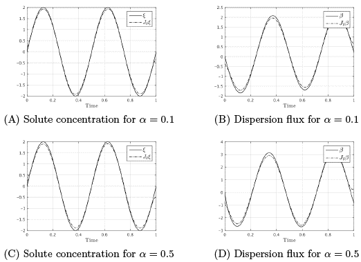
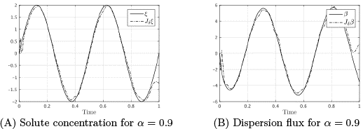
Example 5.2. As a second experiment we solve TFADP (28) with boundary conditions 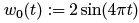 and
and 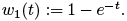
Direct problems (28) and (29) are solved using scheme (27) with parameters h = 1/100 and k = 1 /128, time fractional orders α = 0.10, 0. 50, 0. 90 and noise level ε = 0. 05. Numerical results are presented in Figures (3) and (4).
Further numerical results for parameters h = 1 /50, 1 /100 and k = 1/64, 1 /128, 1 /256, and noise levels ε = 0. 01, 0.05 are listed in Table (4).
6. Final remarks
(1) Problems of the kind TFIADP are relevant in numerical analysis and are potentially useful in different areas of research, including transport problems in groundwater hydrology in the first place.
(2) Discrete mollification with automatic selection of regularization parameters is an appropriate stabilization tool for severely ill-posed TFIADP.
(3) Even knowing that 1-D geometry is adecuate as a first approximation for this inverse problem, an interesting task is to go to dimensions 2 or 3.
(4) Other possible alternatives consists on considering non constant fluid velocity and dispersion coefficients. These changes may lead to nonlinear problems.

