


 Inglés (pdf)
 Articulo en XML
 Referencias del artículo
 Enviar articulo por email
 Citado por SciELO
  Citado por Google
  Similares en
SciELO
Similares en
SciELO  Similares en Google
 Permalink
INTRODUCTION
Sugarcane (Saccharuum spp hybrid), grows in tropical and sub-tropical areas and produces approximately 70% of the world's sugar (Scortecci et al., 2012). In Venezuela, sugarcane grows up in diverse environments. One of the main goals of sugarcane breeding programs is to obtain high-yielding cultivars adapted to different agro-ecological regions (Rea et al., 2014). Therefore, it is essential to establish selection indices that simultaneously combine yield and stability. However, Genotype by Environment Interaction (GEI) reduces the association between genotypic and phenotypic values and affects the selection progress (Rea et al., 2014). The importance of GEI in genotype evaluations and breeding programs has been demonstrated in many crops, including sugarcane. Several statistical methods (parametric and non-parametric) have been proposed to study the GEI (Lin et al., 1986, Mohammadi and Amri, 2008). Becker and León (1988) proposed two concepts for these models: the biological or static, where the ideal genotype will be one that presents minimal variation across environments, showing a constant performance in any area of production (minimum statistical variance), and the agronomic or dynamic that represents an exiguous GEI and is associated with the pretension to obtain an increase in yield in response to environmental improvements.
The most commonly used univariate parametric methods to estimate stability are regression (Eberhart and Russel, 1966), stability variance (Shukla, 1972) and ecovalence (Wricke, 1962). The multivariate model of the Principal Additive Effects and Multiplicative Interactions (AMMI) is based on a linear-bilinear statistical model (Crossa et al., 2004),in which the main effects of genotypes and environments are considered linear terms and are explained by conventional analysis of variance; the bilinear component (non-additive) is imputed to the GEI, and analyzed by the principal component technique. Purchase et al. (2000) developed the AMMI stability value (ASV) using the first two principal components (CP1 and CP2) of the AMMI model.
These parameters are effectively assessing adaptability, but there are cases in which the most adapted genotype does not show good yield. Due to these failures, efforts have been made to develop indices that incorporate both stability and yield in only one criterion to select new cultivars (Rea et al., 2014). Kang and Pham (1991) evaluated several methods for simultaneous selection of yield and stability and proposed the rank-sum that combines the Shukla stability variance and yield in a single value. Bajpai and Prabhakaran (2000) proposed a modified method to rank-sum termed stability index (I). The superiority index (P I ) of Lin and Binn (1988) integrates yield and stability and has been used in selection programs in corn (Zea mays L.), sugarcane, rice (Oryza sativa L.), and soybean (Glicyne max L.).
The practical interest in combining high yields and stability led to the reliability index's development (Annicchiarico, 2002). Farshadfar (2008) , which adds the ASV and yield in a single criterion, suggested an approach known as the genotypic selection index (GSI). The sustainability index (SI) has been used to select stable and high yield in wheat genotypes (Triticum aestivum L.) (Farshadfar et al., 2011).
The objectives of this research were: a) to identify high-yield and stable sugarcane (Saccharum spp., hybrid) genotypes and b) to evaluate the interrelation of stability index and yield.
MATERIALS AND METHODS
Experimental clones. Yield data were obtained from the sugarcane-breeding program at the National Institute for Agricultural Research (INIA), Yaracuy State-Venezuela. The evaluated material consisted of sixteen experimental genotypes: CP80-1743, CP80-1827, CP88-176, CP89-2143, CP89-2377, CP92-1213, CP92-1641, CR83-323, CR87-339, LCP85-384, V90-11, V90-14, V90-2, V90-3, V90-6 and two commercial varieties as control: C323-68 (T) and CP74-2005 (T).
Locations. The genotypes were evaluated in five locations for two years (plant and ratoon crops) in Carora, La Pastora, Turbio I (early growing season), and Turbio II (late growing season) located in Lara state, El Palmar in Aragua state, and Matilde in Yaracuy state. Table 1 shows some agroclimatic characteristics of the localities. Each genotype was planted in three-row plots of 10 m long and 1.5 m wide with three replications in a completely randomized block design. Cultural and agronomic practices prevalent for each environment were applied.
Table 1. Some agroclimatic characteristics of the evaluated localities.
| Locations | rainfall (mm) | Texture | pH |
|---|---|---|---|
| Matilde | 1189 | Silt loam | 8.1 |
| Carora | 1146 | Loam | 7.3 |
| The Palmar | 1115 | Sandy loam | 6.7 |
| Rio Turbio | 700 | Clay loam | 8.0 |
Variable evaluated. The sugarcane was burned, and the plots of each genotype were harvested by hand. A random sample of 10 stems was taken from each plot and weighed. The samples were pressed, and the juice was analyzed to determine the apparent sugar content (Pol% cane).
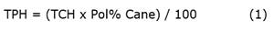
The evaluated variable was cane yield expressed in TPH, which was calculated as a ratio of TCH and Pol% cane by the formula (1) by (Pérez-Guerra et al., 2009):
Statistical analysis. An analysis of variance using the AMMI model was performed to access the variables. Methodologies of adaptability, stability and indices that combine both stability and yield were determined: Genotypic stability index (GSI), stability index (I), reliability index (Ii), geometric adaptability index, rank-sum (RS) and sustainability index (SI). A principal components analysis was performed using the rank of the statistics and indices. The AMMI analysis was carried out according to the model suggested by Crossa et al. (2004) equation 2.

Where:
Yij = Mean yield of ith genotype in the jth environment
μ = the general mean
 = The ith genotypic effect
 = the jth environment effect
n = the number of PCA axes retained in the model
 = eigen value of the PCA axis
 = the ith genotype and jth environment PCA scores for the PCA axis n
€ij= is the residual
Stability methods
Ecovalencia. Wricke (1962) suggested using the GEI for each genotype as a measure of stability which was denominated ecovalence (W).

Where:
 = Observed response of the genotype ;
 = Average of a genotype through environments;
 = mean yield in an environment;
 = grand mean; e = number of environments; a genotype with a low W value is considered high stability.
The stability variance (σi 2) is based on the decomposition of the GEI into g genotypes. It is equal to environmental variance within each environment (σo 2) more environmental variance for each genotype, corrected for additive effects of environments, If σi 2 = σo 2 implies that if σ ́o 2 = 0; then the genotype will be stable.
Variance of Shukla (4)

Where:
 = Observed response of the genotype;
 = average of a genotype through environments;
 = mean yield in an environment;
 = Grand mean; G = number of genotypes; E = Number of environments; low values of variance indicates that a genotype is stable.
AMMI value (ASV). The AMMI Model does not foresee a quantitative measure to estimate stability. Purchase et al., (2000) proposed the value of AMMI (AMMI stability value-ASV). The ASV is the distance from the origin in a dispersion diagram of a two-dimensional system towards the scores of CP1 vs.CP2.
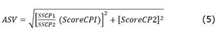
Where: SSCP1 = is the sum of squares of the first principal component (CP1); SSCP2 = is the square sum of the second principal component (CP2); Score CP1 and Score CP2 are the scores of the first two principal components. Low values of ASV in the genotypes are considered widely adapted.
Simultaneous selection for stability and yield
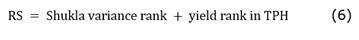
Rank sum (RS). One of the advantages of nonparametric measures is their ease of calculating and interpreting (Rea et al., 2015). This statistic gives equal weight to the rank of yield and variance of Shukla in a single measure. The average genotype’s yield was assigned the rank of 1, and the genotype with the lowest variance of Shukla was imputed the rank of 1. Low values of the rank-sum (RS) indicate better behavior of the genotype (Kang and Pham, 1991).
Genotypic stability index (GSI). This index was recommended by Farshadfar et al. (2011) and is defined as the rank sum of ASV value plus the rank sum of the genotypic mean across the environment.
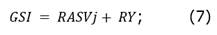
Where: GSI is the stability index for the i th genotype through the environment for TPH; RASVj is the rank of the i th genotype across environment based on the ASV value (AMMI Value); RY i is the rank of the i th genotype based on the average in each environment. Genotypes with low GSI values were considered the best across environments.
Stability index (I). This index was proposed by Bajpai and Prabhakaran (2000) and was computed according to the following equation:
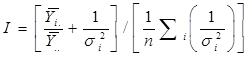 (8)
(8)Where:
 = Average of i
th
genotype;
= Average of i
th
genotype;
 = General mean,
 = Shukla variance of the i
th
genotype. Genotypes with high values of stability indexes are the best.
= Shukla variance of the i
th
genotype. Genotypes with high values of stability indexes are the best.
Superiority index (Pi). The index was calculated from the sum of squares of the differences between the genotype of interest for the genotype of higher yield in each of the environments, so it represents the mean square of the joint effect of genotypes and GEI. In addition, it determines the adaptability in a broad sense (Lin and Binn, 1988) calculated about the maximum response. A small value of Pi implies general adaptation of a genotype. The calculation formula was the following:
 (9)
(9)Where
 = is the mean yield of the i
th cultivar in the j
th environment
= is the mean yield of the i
th cultivar in the j
th environment
 = is the maximum response observed among all the cultivars in environment j.
n = is the number of environments.
Reliability index (Ii). This index was determined following the procedure described by Annichiriaco (2002), based on the distribution of the observed means of TPH across the test environments. The equation used was the following:

Where: mi= mean yield; Si= square root of the environmental variance and Z(P)= Percentile of the normal distribution for a probability value (P). Depending on the level of probability (P), Z (P) can assume the following values: 0.675 to P = 0.75; 0.840 to P =0.80;1.040. P values may vary between 0.95 (for subsistence agriculture in unfavorable cropping regions) to 0.70 for modern agriculture in most favorable regions.
Geometric adaptability index (GAI). The geometric mean can be used as a measure of adaptability:
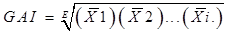 (11)
(11)Where X1, X2 are the mean yields of the first, second and I th genotype through environments and E is the number of environments. Genotypes with high GEI are the chosen ones (Pourdad, 2011).
Sustainability Index (SI). The Sustainability Index was estimated according to the equation used by Babarmanzoor et al. (2009) .
 (12)
(12)Where Y = TPH mean of a genotype through environments
σn= standard deviation
YM = Better yield of a genotype in any year or location
The sustainability index values were divided arbitrarily inside of 5 groups: Very low (until 20 %), Low (21-40 %), moderate (41-60 %), high (61-80%) and very high (plus of 80 %).
Association between statistics, indices and yield. A principal components analysis was performed using the rank matrix to determine the degree of association between indices, statistics and the mean yield in TPH.
RESULTS AND DISCUSSION
AMMI model. The mean yield in TPH was significantly affected by environmental and genotypic effects. The first two axes of the principal components (CP1 and CP2) of the interaction of the AMMI model were significant (p <0.01).
The TPH mean of the locations varied between 14.80 (Turbio I) and 20.56 (Matilde). The yields of the clones ranged from 9.82 (CP92-1641) to 27.92 (CR87-339) (Table 3). Significant differences for the GEI show that the response of the varieties was distinct in diverse environments. Rea et al. (2014) note that the GEI reduces the correlation between genotypic and phenotypic values, affecting selection's progress. One of the methods to minimize the GEI is to select stable cultivars using stability analysis.
Table 3. Average yield in TPH of eighteen sugarcane genotypes at six environments in two cycles of harvest.
| Variety | Carora | Palmar | Matilde | La Pastora | Turbio I | Turbio II | Mean |
|---|---|---|---|---|---|---|---|
| C 323-68 (T) | 19.90 | 23.61 | 22.74 | 22.88 | 17.35 | 17.72 | 20.70 |
| CP74-2005 (T) | 15.39 | 21.85 | 23.22 | 15.99 | 15.71 | 15.91 | 18.01 |
| CP80-1743 | 13.62 | 16.13 | 22.90 | 19.22 | 15.22 | 17.27 | 17.39 |
| CP80-1827 | 10.54 | 15.49 | 18.47 | 21.86 | 10.92 | 14.13 | 15.23 |
| CP88-1762 | 13.32 | 15.01 | 19.36 | 17.37 | 12.64 | 13.43 | 15.19 |
| CP89-2143 | 18.13 | 16.59 | 21.50 | 20.77 | 15.38 | 12.98 | 17.56 |
| CP89-2377 | 13.64 | 16.14 | 16.99 | 20.88 | 13.97 | 10.38 | 15.33 |
| CP92-1213 | 11.31 | 16.06 | 20.21 | 21.21 | 10.75 | 13.72 | 15.54 |
| CP92-1641 | 9.82 | 14.56 | 14.90 | 13.52 | 11.02 | 10.67 | 12.41 |
| CR83-323 | 18.30 | 17.34 | 19.70 | 18.27 | 15.64 | 17.20 | 17.74 |
| CR87-339 | 25.42 | 27.92 | 27.56 | 25.91 | 24.15 | 23.52 | 25.75 |
| LCP85-384 | 16.10 | 18.52 | 20.05 | 18.27 | 15.85 | 13.11 | 16.98 |
| V90-11 | 14.57 | 16.74 | 24.19 | 19.65 | 13.78 | 15.83 | 17.46 |
| V90-14 | 12.19 | 14.59 | 16.91 | 16.75 | 14.26 | 11.07 | 14.30 |
| V90-2 | 13.63 | 17.24 | 19.91 | 14.08 | 12.27 | 20.75 | 16.31 |
| V90-3 | 18.63 | 15.51 | 20.57 | 17.92 | 13.93 | 16.85 | 17.23 |
| V90-6 | 14.54 | 15.70 | 19.70 | 17.98 | 14.20 | 14.39 | 16.09 |
| V98-76 | 15.94 | 16.45 | 21.14 | 18.01 | 19.44 | 16.31 | 17.88 |
| Mean | 15.28 | 17.52 | 20.56 | 18.92 | 14.80 | 15.29 | 17.06 |
(T)= Checks
Yield stability in TPH. Table 4 shows the results of several statistics and stability indices. For the ecovalence and variance of Shukla, the most stable genotypes were CP88-1762, V90-6 and CP92-1641. This similarity in the results of both methods has been demonstrated by Becker and León (1988) . The AMMI stability value was estimated according to Purchase et al. (2000) . The results showed that the sum of squares of the first two principal components explained 67% of the data variance. According to the ASV, the genotypes V90-6, CP88-1762 and CP92-1641 are the most stable, coinciding with the genotypes selected by the ecovalence and Shukla variance methods. Purchase et al. (2000) point out that ASV can be compared with W and σ i 2.
Indices for stability and yield
Kang’s (1988) rank-sum. The results of six stability indices are presented in Table 4. According to Kang's rank-sum, genotypes with low values are considered the most desirable. This index revealed that the genotypes CR 87-339 and C32-368 (T) had the lowest values and therefore were the most stable and yielding, while those with high values such as the genotypes: CP80-1827, V90-2, CP89-2377, CP92-1213 were the most unstable.
Table 4. Indices for simultaneous selection of stability and yield in eighteen sugarcane genotypes evaluated in six environments.
| Genotipos | TPH | (W) | σi2 | Score CP1 | Score CP2 | ASV | RS | I | P i | Ii | GAI | SI (%) | GSI |
|---|---|---|---|---|---|---|---|---|---|---|---|---|---|
| C 323-68 (T) | 20.7 | 35.5 | 7.3 | 0.7 | 1.38 | 1.5 | 9 | 0.04 | 161.2 | 16.6 | 20.7 | 66.8 | 6 |
| CP 74-2005 (T) | 18.0 | 90.6 | 19.7 | -3.2 | 0.62 | 4.5 | 19 | 0.03 | 383.9 | 13.5 | 17.7 | 54.2 | 17 |
| CP 80-1743 | 17.4 | 41.1 | 8.5 | -0.7 | -2.8 | 2.9 | 17 | 0.03 | 463.6 | 13.1 | 17.2 | 53.6 | 19 |
| CP 80-1827 | 15.2 | 107.9 | 23.6 | 3.9 | -4.1 | 6.8 | 35 | 0.03 | 738.2 | 10.2 | 14.7 | 42.5 | 31 |
| CP 88-1762 | 15.2 | 3.2 | 0.01 | 0.3 | -0.61 | 1.0 | 17 | 5.66 | 703.4 | 10.3 | 15.0 | 48.2 | 18 |
| CP 89-2143 | 17.6 | 52.6 | 11.1 | 2.4 | 2.02 | 3.9 | 17 | 0.03 | 432.4 | 13.5 | 17.3 | 61.1 | 19 |
| CP 89-2377 | 15.3 | 84.1 | 18.2 | 4.8 | 1.84 | 6.9 | 28 | 0.03 | 690.7 | 11.3 | 14.9 | 50.3 | 31 |
| CP 92-1213 | 15.5 | 84.9 | 18.4 | 3.5 | -3.93 | 6.2 | 28 | 0.03 | 691.5 | 10.7 | 15.3 | 46.2 | 28 |
| CP 92-1641 | 12.4 | 17.5 | 3.2 | -0.6 | 0.77 | 1.1 | 21 | 0.03 | 1073.1 | 8.6 | 12.3 | 52.5 | 21 |
| CR 83-323 | 17.7 | 35.7 | 7.3 | -1.9 | 1.44 | 2.9 | 13 | 0.03 | 394.9 | 14.6 | 17.7 | 71.2 | 15 |
| CR 87-339 | 25.8 | 34.2 | 6.9 | -1.3 | 2.61 | 3.2 | 7 | 0.05 | 0.0 | 21.4 | 25.7 | 73.6 | 13 |
| LCP 85-384 | 16.9 | 24.5 | 4.8 | 0.5 | 2.57 | 2.7 | 14 | 0.03 | 467.2 | 12.7 | 16.8 | 54.1 | 16 |
| V 90-11 | 17.5 | 45.7 | 9.6 | 0.3 | -2.74 | 2.8 | 17 | 0.03 | 459.7 | 12.8 | 17.1 | 49.3 | 15 |
| V 90-14 | 14.3 | 24.9 | 4.9 | 1.3 | 1.8 | 2.6 | 22 | 0.03 | 802.5 | 11.4 | 14.8 | 64.3 | 22 |
| V 90-2 | 16.3 | 178.5 | 39.4 | -6.7 | -3.43 | 9.8 | 29 | 0.03 | 600.7 | 11.5 | 16.0 | 51.1 | 29 |
| V 90-3 | 17.2 | 57.9 | 12.3 | -1.9 | 0.51 | 2.7 | 21 | 0.03 | 461.6 | 12.6 | 17.1 | 56.9 | 16 |
| V 90-6 | 16.1 | 2.8 | 0.09 | 0 | 0.1 | 0.1 | 14 | 0.34 | 574.5 | 12.1 | 15.9 | 57.6 | 13 |
| V 98-76 | 17.9 | 63.8 | 13.6 | -1.5 | 1.96 | 2.8 | 17 | 0.03 | 399.2 | 14.1 | 17.8 | 63.4 | 13 |
(T)= Checks
Stability index (I). The basic element in the index construction is that the genotypes’ achievement levels and their stability are quantified by the individual achievement expression relative to the average behavior of the group of genotypes evaluated.Bajpai and Prabhakaran (2000) proposed this index arguing that the rank sum method has its weaknesses due to the heavyweight given to yield. The ranks assigned by the stability index were in increasing order, the genotype with the highest stability index (I) received the rank 1, and the lowest index received the rank 14 of the 18 genotypes evaluated. According to this index, the CP88-1762, V90-6, CR87-339 and C323-68 genotypes were the most stable and CP80-1827, CP89-2377 and CP92-1213 the adapted less.
Linn and Binn superiority index (Pi). This index is a unique measure of stability and yield. Based on this method, the selected genotypes were those with low indices and yields above the general average (Kilic et al., 2010). In this case, the best genotypes were C87-339, C323-68, CP74-2005 (T), CR83-323 and V98-78.
Geometric adaptability index (GAI). This index is based on the geometric mean of the genotype. Genotypes with high GAI values are acceptable (Pourdad, 2011). In this case, the genotypes CR 87-339, C323-68 (T), V98-76 and CR 83-323 were those with the best yields and stability.
Reliability index (Ii). To estimate this index, it was assumed that the technological level for agriculture of Venezuela falls between subsistence levels and modern agriculture, where it was taken (P) = 0.8 corresponding to a value of Z (p) = 0.84. This value was inserted in the equation of Ii; a genotype is selected if it has high values of Ii. In this way, the genotypes: CR87-339, C323-68, CR83-323 and V98-76 were the most outstanding. Gómez-Becerra et al. (2007) selected genotypes of wheat (T.Aestivum) based on this method.
Sustainability Index (SI). The values of this index were arbitrarily divided into five groups, from very low and very high. The genotypes in the high group (61-80%) of sustainability were CR87-339, CR83-323, C323-68, V90-14, V98-76, CP89-2143. The rest of the genotypes were grouped as of moderate sustainability. This index was used successfully by Koli and Prakash (2013) in the selection of rice varieties.
Genotypic stability index (GSI). This index integrates both the AMMI value and the yield in a single selection criterion proposed by Fardshafar (2008). The genotypes with low values of this index are those selected. According to this criterion, the genotypes with the best behavior were C323-68, CR87-339, V98-78 and V90-6.
In the results obtained, it can be observed that when only the stability methods are used, the selected genotypes are not the ones with the best yields; On the other hand, when the selection indices are used, the most yielding genotypes appear among those selected: CR87-339 and C32-362. This demonstrates the importance of considering both stability and yield selecting genotypes when they are evaluated in diverse environments.
Association between different indexes using main components. An analysis of the principal components of the matrix of ranks of statistics and stability indexes was made to observe the associations between them (Table 5). A biplot with the values of CP1 and CP2 is shown in figure 1. The two principal components represented 90.8% of the total variation, distinguishing the indices in three different groups. In group 1 (G1) were located P i , GAI, Ii and the yield in TPH. This group coincided in classifying genotypes CR87-339, C323-68 and V98-76 as the most stable and best performing. The second group (G2) was composed of RS, I, SI and GDI and identified the genotypes CR87-339 and C323-68 as the best. The genotype V98-76 was selected by the GDI and SI indices. The W statistics, Shukla and the AMMI value constituted the third group (G3). According to the statistics, the best genotypes were CP87-1762, V90-6 and CP 9216-41. Group 3 differed in the classification of genotypes to the groups 1 and 2. This is a clear indication of the utility of using indices where both yield and stability are considered in a single criterion. The statistics of Group 3 only measure stability, and there are cases in which the most stable genotype is not the most yield (Mohammadi and Amri, 2008). These results corroborate the findings of other authors searching for approaches that include both stability and yield in a single index for cultivars selection in different environments (Babarmanzoor et al, 2009; Farshadfar et al, 2011; Rao and Prabhakaran, 2005).
Table 5. Ranks of sugarcane genotypes according to the mean of TPH, stability and stability indexes.
| Genotipos | TPH | W | σi2 | ASV | RS | I | P i | Ii | GEI | SI | GSI |
|---|---|---|---|---|---|---|---|---|---|---|---|
| C323-68 | 2 | 7 | 7 | 4 | 2 | 4 | 2 | 2 | 2 | 3 | 1 |
| CP74-2005 | 3 | 16 | 16 | 14 | 11 | 11 | 3 | 6 | 4 | 9 | 9 |
| CP80-1743 | 8 | 9 | 9 | 11 | 6 | 7 | 8 | 7 | 7 | 11 | 11 |
| CP80-1827 | 15 | 17 | 17 | 16 | 18 | 18 | 16 | 17 | 17 | 18 | 17 |
| CP88-1762 | 16 | 1 | 1 | 2 | 6 | 1 | 15 | 16 | 14 | 16 | 10 |
| CP89-2143 | 6 | 11 | 11 | 13 | 6 | 7 | 6 | 5 | 6 | 6 | 11 |
| CP89-2377 | 14 | 14 | 14 | 17 | 15 | 16 | 13 | 14 | 15 | 14 | 17 |
| CP92-1213 | 13 | 15 | 15 | 15 | 15 | 16 | 14 | 15 | 13 | 17 | 15 |
| CP92-1641 | 18 | 3 | 3 | 3 | 12 | 13 | 18 | 18 | 18 | 12 | 13 |
| CR83-323 | 5 | 8 | 8 | 10 | 3 | 6 | 4 | 3 | 5 | 2 | 5 |
| CR87-339 | 1 | 6 | 6 | 12 | 1 | 3 | 1 | 1 | 1 | 1 | 2 |
| LCP85-384 | 10 | 4 | 4 | 6 | 4 | 5 | 10 | 9 | 10 | 10 | 7 |
| V90-11 | 7 | 10 | 10 | 8 | 6 | 7 | 7 | 8 | 8 | 15 | 5 |
| V90-14 | 17 | 5 | 5 | 5 | 14 | 13 | 17 | 13 | 16 | 4 | 14 |
| V90-2 | 11 | 18 | 18 | 18 | 17 | 15 | 12 | 12 | 11 | 13 | 16 |
| V90-3 | 9 | 12 | 12 | 7 | 12 | 11 | 9 | 10 | 9 | 8 | 7 |
| V90-6 | 12 | 2 | 2 | 1 | 4 | 2 | 11 | 11 | 12 | 7 | 2 |
| V98-76 | 4 | 13 | 13 | 9 | 6 | 7 | 5 | 4 | 3 | 5 | 2 |


