


 English (pdf)
 Article in xml format
 Article references
 Send this article by e-mail
 Cited by SciELO
  Cited by Google
  Similars in
SciELO
Similars in
SciELO  Similars in Google
 Permalink
INTRODUCTION
In conventional agriculture, a large percentage of crop yield variability is due to the differentials that may exist in the soil properties (Bramley, 2009). This variability can be analyzed from different perspectives, scales based on both the intervention objectives and the level of decision required. It also depends on natural disturbances and human actions, especially in agricultural practices (Fraterrigo & Rusak, 2008).
Mapping, the use of cartographic tools, is a valuable approach to adapt work processes to landscape changes. Mapping is referred to as a tool because it is an important means to strengthen decision making, in this case, to improve agricultural production through nutrient use efficiency (NUE) (Murillo, 2006).
The recognition of the role of fertilizers in increasing agricultural production, and consequently, in the production of food, fiber, and even energy, contrasts severely with the negative nature of the information that is currently being released on fertilizers use (Murillo, 2006).
For agricultural sciences, information at different scales is often used to support decision making with respect to diagnosis, monitoring, and predictions related to the management of productive systems (Pachepsky & Hill, 2017). At the research level, the spatial variability of physical and chemical properties of soils at the field scale has been more widely considered than the patterns of such distribution (Reza et al., 2017). In this sense, the modeling of these properties will allow, among others, to estimate the distance in which different soil samples are independent as well as to improve the sampling process either for planning activities in a traditional way or under a precision agriculture scheme (Peralta & Costa, 2013; Peralta et al., 2015).
In terms of production and academic contributions, various activities are carried out in most production units. Regarding Botana Experimental Farm of Universidad de Nariño - Colombia, is a site where different activities take place, including growth, development, and productivity assessment of certain crops from the Andean region. In each of these, physical and chemical studies of the soils are generally conducted to determine their fertility level, which benefits the crop or system under study.
However, in most of the agricultural production units in the region, the results of soil analysis are not very useful over time. One of the reasons that account for this is the fact that the analyses are not properly stored or processed in databases, which hinders production planning in the long run. If properly used, these databases or mapping, which depict the spatial distribution of the physical and chemical properties of soils, would make it possible to estimate the productive potential of the farm. This would result in appropriate agricultural, forestry, and livestock planning, without the need to repeat the already executed processes.
According to Álvarez et al. (2015), today, several research centers are using geographic information systems (GIS) to elaborate soil maps, which are of vital importance for planning and correct soil management. In turn, appropriate management increases the competitive capacity of soils and the possibilities to better channel agricultural and agroforestry programs and projects. Using GIS, soil fertility zonation studies facilitate adequate planning in terms of agricultural use of soil and its optimal management (Álvarez et al., 2015). Similarly, these tools allow making timely recommendations that would permit the optimization of resources and the definition of productive systems that become a very important input for farm management and thus take measures that promote the implementation of Precision Agriculture in these research centers.
Site-specific fertilization involves the assessment of the spatial relationships between soil properties and crop yield. In this sense, the spatial distribution of physical, chemical, and biological parameters of soil has been observed to affect crop yield (Machado et al., 2000). However, the spatial dependence of soil biological parameters has been little explored (Moreno, 2011). One of the most important uses of GIS is spatial analysis, especially the use of interpolations of different types of variables. In agriculture, the use of this tool makes it possible to analyze the variability of different characteristics in the landscape such as soil, diseases, and pests, among others (Clay et al., 2007). This undoubtedly helps to quantify the impact of this variation on production and the possible management guidelines required to optimize farm yields (Bertsch et al., 2002).
Considering the above, this research aimed to assess the implementation of soil fertility zoning at Botana Experimental Farm of Universidad de Nariño as a tool to contribute to productive processes, research, and academic practices of the agriculture programs of the University and productive systems of the region.
MATERIALS AND METHODS
Location. The present study was carried out at Botana Experimental Farm of Universidad de Nariño - Department of Nariño, at 2820 m asl, 12.4ºC and an average annual rainfall of 694mm. It is located in a low mountain dry forest life zone (bs-MB) at 1°09'30.8"N; 77°16'31.8"W.
Fieldwork and laboratory methodology. Through the use of a Geographic Information System, a sampling grid of 0.5 hectares was established, for a total of 106 soil samples in the productive areas of Botana Experimental Farm. That is, the samplings were drawn from an overall area of 55 hectares (productive area). This aspect guaranteed the significance of the study area about the established interpolation method and the areas dedicated to production within the system.
Once the sampling grid was defined, the sampling points were identified and 15 soil subsamples were taken in each grid using an Edelman auger. These subsamples were mixed into a single sample, placed in plastic bags and labeled. The samples were sent to the laboratory of Universidad de Nariño to determine their physical-chemical characteristics (Table 1 and Table 2).
Table 1 Chemical parameters analyzed in the samples.
| Essays | Method | Technique | U. of measure |
|---|---|---|---|
| pH, potentiometer Soil: Water Ratio (1: 1) | NTC 5264 | Potentiometric | |
| Walkley- Black (Colorimetric) - NTC 5403 | Spectrophotometric uv-vis | % | |
| Organic mater | Bray II y Kurtz NTC 5350 | Spectrophotometric uv-vis | mg/Kg |
| Available phosphorus | CH3COONH4 1NpH7 NTC 5268 | Volumetric | cmol+ / Kg |
| Cation Exchange Capacity (CEC) | CH3COONH4 1NpH7 NTC 5349 | Atomic absorption spectrophotometry | |
| Exchange calcium | |||
| Magnesium Exchange | |||
| Exchange Potassium | Extracción KCl 1N NTC 5263 | Volumetric | |
| Shift Aluminum | DTPA - NTC 5526 | Atomic absorption spectrophotometry | mg/Kg |
| Available iron | |||
| Manganese available | |||
| Copper available | |||
| Zinc available | Hot water NTC 5404 | Spectrophotometry uv-vis | |
| Boron available | Based on organic matter | Calculation | % |
| Total Nitrogen | Walkley- Black (Colorimetric) NTC5403 | Spectrophotometry uv-vis | % |
| Organic carbon | (Ca (H2P04) 2.H20) 0,008M NTC 5402 | Spectrophotometry uv-vis | mg/Kg |
Table 2 Physical parameters analyzed in the samples.
| Essays | Method | Technique | U. of measure |
|---|---|---|---|
| Texture | Touch | Textural grade | |
| Bulk density | Graduated cylinder | Gravimetric | g/cc |
Statistical and geostatistical analysis. The data were descriptively analyzed and a principal component analysis was performed using the SPAD software. The geostatistical analysis was carried out with ArcGIS 10 software (ArcGIS, 2010). The semivariogram was obtained for each characteristic and through an iterative process where the active lag and the step were modified; the theoretical model of best fit was established, taking into account as parameters of decision the coefficient of determination (R2) and the sum of squares of the residuals (RSS). Subsequently, a cross-validation analysis was carried out, of importance in the estimation of values in unsampled sites, through the point Kriging interpolation method, because the samples come from points and not from combinations or mixtures (Balzarini, 2014). This interpolation was the basis for the construction of thematic maps that allow visualizing the spatial variability of each of the physical and chemical properties analyzed. In the mentioned software, spatial distribution maps were also made for each variable, subsequently reclassifications of the results were performed to generate other fertility distribution maps for each variable in the three ranges, according to the values for the Andean region (Table 3).
Table 3 Interpretation of results (ICA, fertilization in various crops, fifth approximation).
| Bases | cmol+/Kg | Phosphorus and minor elements | mg/Kg | pH | |||||
|---|---|---|---|---|---|---|---|---|---|
| Low | Medium | High | Low | Medium | High | Value | Category | ||
| Ca | < 3 | 03-jun | > 6 | P | < 20 | 20 - 40 | > 40 | < 5.5 | Extremely acidic |
| Mg | < 1.5 | 1.5 - 2.5 | > 2.5 | Fe | < 25 | 25 - 50 | > 50 | 5.5 - 5.9 | Moderately acidic |
| K | < 0.2 | 0.2 - 0.4 | > 0.40 | Mn | < 5 | 05 | > 10 | 6.0 - 6.5 | Suitable |
| Organic matter according to climate (%) | Cu | < 2 | 02 | > 3 | 6.6 - 7.3 | Neutral | |||
| Cold | < 5 | 5 -10 | > 10 | Zn | < 1.5 | 1.5 - 3 | > 3 | 7.4 - 8.0 | Alkaline |
| Half | < 3 | 3-5 | > 5 | B | < 0.2 | 0.2 - 0.4 | > 0.4 | > de 8 | Very alkaline |
| Warm | < 2 | 2-3 | > 3 | S | < 10 | -20 | > 20 | ||
RESULTS AND DISCUSSION
General statistics. When analyzing the soil fertility traits of the total area samples, a high percentage of variation was found, which suggested that there was a high intrazonal variability (Table 4).
Table 4 General statistics of the soil fertility variables at Botana Experimental Farm.
| Variable | Half | Median | D.E. | Var (n) | CV | Mín | Máx | Asymmetry | Kurtosis |
|---|---|---|---|---|---|---|---|---|---|
| pH | 5.67 | 5.63 | 0.44 | 0.2 | 7.84 | 4.54 | 7.04 | 0.64 | 0.82 |
| MO | 5.23 | 4.59 | 2.16 | 4.6 | 41.24 | 1.88 | 14.7 | 1.42 | 2.83 |
| P | 62.04 | 21.85 | 98.41 | 9593.7 | 158.62 | 4.34 | 611.0 | 3.64 | 15.79 |
| CIC | 20.71 | 20.4 | 6.44 | 41.08 | 31.09 | 10.7 | 37.9 | 0.58 | -0.24 |
| Ca | 7.51 | 6.83 | 2.6 | 6.67 | 34.55 | 0.05 | 15.3 | 0.89 | 1.43 |
| Mg | 3.3 | 3.07 | 1.22 | 1.47 | 36.93 | 1.38 | 8.7 | 1.54 | 3.53 |
| K | 0.9 | 0.68 | 0.85 | 0.71 | 94.13 | 0.0 | 5.37 | 2.25 | 7.33 |
| Fe | 273.92 | 264.0 | 68.31 | 4622.21 | 24.94 | 142.0 | 395.0 | -0.06 | -1.07 |
| Mn | 28.62 | 25.2 | 16.74 | 277.64 | 58.5 | 3.6 | 90.6 | 0.86 | 1.09 |
| Cu | 3.11 | 2.86 | 1.93 | 3.71 | 62.22 | 0.17 | 14.5 | 2.95 | 12.76 |
| Zn | 5.82 | 3.16 | 8.55 | 72.39 | 146.94 | 0.17 | 55.0 | 3.86 | 16.19 |
| B | 0.19 | 0.14 | 0.1 | 0.01 | 50.09 | 0.06 | 0.63 | 2.35 | 6.23 |
| N | 0.46 | 0.18 | 2.7 | 7.23 | 585.59 | 0.07 | 28.0 | 10.28 | 100.83 |
| C | 3.03 | 2.66 | 1.25 | 1.55 | 41.22 | 1.09 | 8.51 | 1.42 | 2.8 |
| S | 6.55 | 5.83 | 4.75 | 22.36 | 72.57 | 2.55 | 46.4 | 5.96 | 45.25 |
| DAP | 0.89 | 0.89 | 0.09 | 0.01 | 10.22 | 0.6 | 1.06 | -0.61 | 0.43 |
Taking into account some classifications for this type of results in similar studies, such as the one carried out by Vásquez (2009), we can classify the variability of the data as follows:
Relatively low or homogeneous variations are only presented for pH and bulk density (DBH), as shown in Table 5, whose similar results were obtained in a study of the variability of soil fertility of the experimental farm of the University of Magdalena (Vásquez, 2009). There is also agreement with the results found by Henríquez (2013), Londoño & Moreno (2014) and Ibarra et al. (2009).
Table 5 Classification of the variability of the soil fertility parameters at Botana Experimental Farm.
| Category of variables | Variability coefficient (CV) | Traits |
|---|---|---|
| Relatively homogeneous | < 20 | DAP, pH |
| Moderately heterogeneous | 20-40 | CIC, Ca, Mg, Fe. |
| Normally heterogeneous | 40-60 | MO, Mn, B, C. |
| Extremely heterogeneous | >60 | P, K, Cu, Zn, N, S. |
Source: Vásquez (2009).
The traits that presented extremely heterogeneous variability were P, K, Cu, Zn, N and S. These results also coincide with what was found by Londoño & Moreno (2014). Likewise, Gutiérrez et al. (2010), Moreno (2011) and Alesso et al. (2017) found in a soil fertility distribution study that available phosphorus and potassium showed high coefficients of variation. Moreno (2011) argues that although pH is a factor that influences the availability of phosphorus in the soil, he did not find a relationship between the high variability shown by this element and the low coefficients of variation observed in pH.
The high value of the coefficient of variation for P (158%) agrees with several works reported in the literature. In this sense, Molina et al. (2005) cite similar results. While the following: Ovalles (1991); Paz et al. (1996); Melchiori & Echeverría (2000), Ponce et al. (1999); Sadeghian et al. (2001); Jaramillo (2002) and Silva et al. (2003), say it may be due to residuality due to fertilization with P.; and that other factors influencing phosphorus retention by the soil, such as: a) Organic matter. In general, it has been found that the effect that the organic phase of the soil P-S diminishes the fixation of phosphorus. b) Presence of hydrated iron and aluminum oxides. In acid soils, these abound and form insoluble compounds with phosphorus. e) Amount and type of clay.
Geostatistical analysis of soil fertility. An exploratory data analysis was performed using the Infostat software, applying a basic statistic to identify the mean, variance, standard deviation, kurtosis and skewness of the data. The SPAD software was applied for multivariate analysis to determine the explanatory traits of the main soil components. In the ArcGIS 10 program, the geostatistical analysis was performed (ArcGIS, 2010). For each trait, the semivariogram was obtained, and through an iterative process in which the active lag and the step were modified. A theoretical model of best fit was established, taking into account as decision parameters the coefficient of determination (R2) and the sum of squares of the residuals (RSS), for which the first must be the closest to 100% and the second the smallest within the situations raised. The parameters of the best-fit theoretical semivariograms obtained for each of the properties studied are recorded in Table 6.
Table 6 Parameters of the semivariograms for the fertility variables using the Kriging model.
| Variable | Model | Nugget effect Co | Sill Co+C | %C0/ | Effective Range (m) | Root-Mean-Square | Root-Mean-Square Standardized | Average Standard Error | Dependence |
|---|---|---|---|---|---|---|---|---|---|
| (C0+C) | |||||||||
| pH | Spherical | 0.02 | 0.21 | 9.5 | 325 | 0.26 | 0.97 | 0.27 | Strong |
| MO | Gaussian | 0.03 | 0.04 | 75 | 91.3 | 1.36 | 0.89 | 1.48 | Moderate |
| P | Gaussian | 0.3 | 0.67 | 44.8 | 305.3 | 40.7 | 1.39 | 51.9 | Moderate |
| CIC | Spherical | 0.02 | 0.013 | 153.8 | 263.2 | 3.85 | 1.01 | 4.05 | Weak |
| Ca | Gaussian | 0.01 | 0.25 | 4 | 74.2 | 2.47 | 1.77 | 3.95 | Strong |
| Mg | Exponential | 0.018 | 0.05 | 36 | 82 | 0.93 | 0.9 | 0.96 | Moderate |
| K | Gaussian | 0.15 | 0.76 | 19.7 | 97.6 | 0.55 | 1 | 1.14 | Strong |
| Fe | Spherical | 0.007 | 0.06 | 11.7 | 373 | 39.6 | 0.92 | 44.9 | Strong |
| Cu | Gaussian | 0.09 | 0.16 | 56.3 | 342 | 1.47 | 1.17 | 1.21 | Moderate |
| Zn | Spherical | 0.65 | 0.47 | 138.3 | 355 | 2.9 | 0.95 | 4.44 | Weak |
| B | Spherical | 0.03 | 0.06 | 50 | 376 | 0.05 | 1.17 | 0.04 | Moderate |
| N | Spherical | 0.01 | 0.03 | 33.3 | 78.5 | 0.04 | 1.02 | 0.04 | Moderate |
| C | Spherical | 0.01 | 0.04 | 25 | 78 | 0.74 | 0.96 | 0.78 | Strong |
| S | Gaussian | 0.07 | 0.05 | 140 | 208 | 2.1 | 0.97 | 2.17 | Weak |
| Textura | Exponential | 0.09 | 0.05 | 180 | 71.5 | 1.27 | 0.87 | 1.48 | Moderate |
Nugget: variance of spatial discontinuity due to measurement error or micro variability. Sill: maximum threshold of the semi-variance. Range Ao: range of spatial dependence where the sill is reached.
The models of the selected semivariograms correspond to those with the greatest spatial adjustment that explain the distribution of the evaluated variables. Table 6 shows that the semivariograms with the spherical model are the best fits for CIC, Fe, Zn, B, N and C. For MO, P, Ca, K and S, it was the Gaussian, and for Mg and texture, the Exponential model corresponded.
The range indicates the distance from which the samples are spatially independent of each other, and represents the size of grain or stain that the variable represents; in this sense, the traits with the greatest scope of spatial dependence were pH, P, Zn and B. On the other hand, the traits with the minor spatial dependence were Ca, Mg, N, C and texture. It is also observed in Table 6 that in all cases, the effective range exceeded the minimum sampling distance used in this study, which was 50m, suggesting an adequate sampling distance (Van et al., 2000).
The spatial dependence was analyzed through the relative Nugget effect [%C0 / (C0 + C)], cited by Trujillo (2011). That revealed a strong dependence for pH, Ca, K, Fe and C (<25%), while MO, P, Mg, Cu, B, N and texture have a moderate dependence (25-75%) and weak spatial dependence (> 75%) for CIC, Zn and S.
Spatial distribution maps. According to Balzarini (2014), Kriging interpolations allow the generation of spatial distribution maps for each of the physical and chemical traits studied. As an example, the spatial distribution maps for soil organic matter (SOM) and Mg are indicated below in Figure 1.
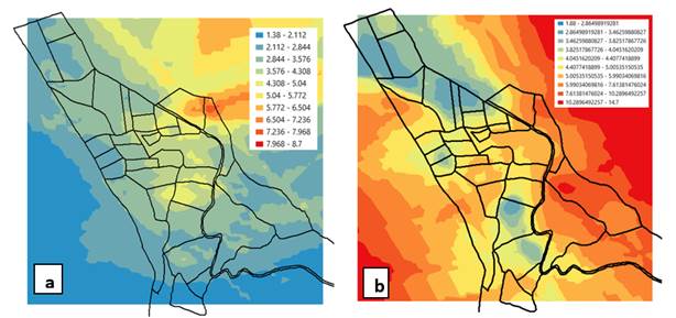
Figure 1 Interpolation of the spatial distribution according to the Kriging method for SOM (a) and Mg (b).
Considering the samplings carried out and the interpolation of the evaluated variables, Figures 2 and Figure 3 show the values reclassified according to the fertility ranges for the Andean zone mentioned in Table 3 of this document. First, Figure 2 indicates the spatial distribution for Boron B, Calcium Ca, Carbon C, Cation Exchange Capacity CIC, Copper Cu, Potassium K and Magnesium Mg, while Figure 3 shows the corresponding values for Manganese Mn, Organic Matter SOM, Nitrogen N, Phosphorus P, Zinc Zn, pH and Texture. In this way, maps with high, medium and low ranges were generated for the said traits. From the data observed in the maps, it is inferred that variables such as Mg, Mn, Ca and K occupy most of the surface of Botana Experimental Farm in a high range, both distributed in the upper, middle and lower part of the farm. The Cu and P presented a certain range, especially towards the middle and lower zones. The variables B, C, N and MO, did not present high ranges, only medium and low.
According to the texture data obtained (Figure 3), the vast majority of the soils of Botana Experimental Farm (12ha) have a sandy clay loam to clay loam texture, and only 5ha are of a sandy loam to loamy texture. The thematic map for pH (Figure 3) shows areas ranging from red (neutral) to green (very strongly acidic). In general, most of the farm has moderately acidic soils (16has).
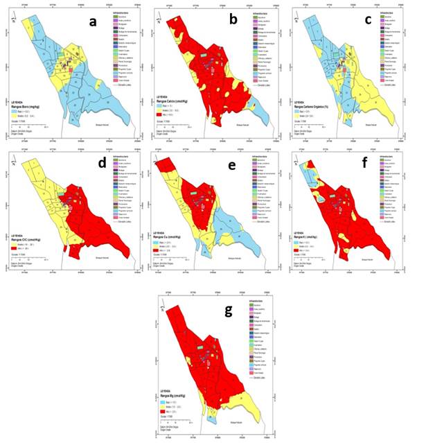
Figure 2 Classification of spatial distribution of B (a), Ca (b), C (c), CIC (d), Cu (e), K (f) and Mg. The colors red, blue and yellow represent high, medium and low contents, respectively.

Figure 3 Classification and spatial distribution of Mn (a), SOM (b), N (c), P (d), and Zn (e). Where the red, blue, and yellow colors represent high, medium and low content of the evaluated variables, respectively; For pH (f), where red for pH represents values greater than 6.5 and green less than 5.0; For Texture (g), red represents sandy loam to loam soils, dark green loam to clay loam, orange clay loam, and light green sandy clay loam.
Classification analysis. To define relatively homogeneous zones based on the principal components, the first three components were selected, explaining 80% of the variability of the data. This analysis allowed obtaining three clusters (Figure 4).
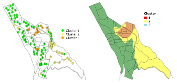
Cluster 1. Making an interpolation of the sampled points that correspond to this group, an area of 20.7has was obtained, located towards the western side of Botana Experimental Farm, which corresponds to the lots: 1, 2, 3, 4, 5, 6, 7, 11, 12, 13, 14, 15, 16, 17, 18, 20, 21, 22, 32, 24, 35, 26 and 27. The traits of these batches are: high content of Mg, K, Zn, Mn and Ca; low C and SOM content; medium to low P and Cu content; medium CEC; moderately acidic pH, and sandy clay loam to loam texture.
Cluster 2. This group corresponds to an area of 13.9has, located towards the eastern part of the farm, which corresponds to lots: 28, 29, 30, and 31, part of 32, 7 and 11. The traits of this cluster are strongly acidic pH; medium SOM content; low content of P, B, Cu; high content of K, C, Ca, Mg, Mn; high CIC; texture Sandy Clay Loam to Sandy Loam.
Cluster 3. This group corresponds to an area of three hectares, located towards the southeastern part of Botana Experimental Farm. The traits of this zone are neutral pH; medium content of B; high content of Zn, K, P, Ca, Cu, Mg, Mn; high CEC; low C content; texture Sandy Clay Loam to Clay Loam.
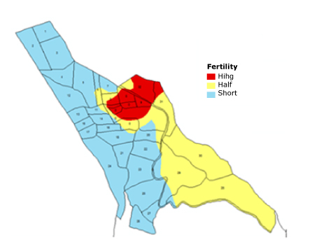
According to the previous characteristics, we can assure them that the third cluster presents the best conditions; therefore, it corresponds to an area of high fertility. It should be noted that the administrative infrastructure of the farm is located in this area; however, there are many agricultural vocations with good fertility traits. The second Cluster presents quite favorable conditions for the development of cold-climate crops; therefore, it corresponds to a zone of medium fertility. The first Cluster presents quite limiting traits since it presents the lowest content in some elements, such as SOM, Cu, C and P, with a loamy-to-loamy sandy clay texture (Figure 5).
CONCLUSIONS
In general, the properties evaluated, except for pH and bulk density, showed significant variability and spatial distribution throughout the study area. Mg, Mn, Ca and K occupy most of the surface, while organic matter and phosphorus content are the most limiting properties. In this case, the distribution maps made it possible to identify spatial trends that, independently of signifying a specific fertility level, could be projected as references for differential nutrition actions in farm management.
Based on the restriction levels for the evaluated traits and possibly due to the soil mineralogy dominated by non-crystalline aluminosilicates, the low cation exchange capacity and soil management factors, three fertility zones could be identified on the farm: high, medium and low, the latter being the most predominant.

