


 English (pdf)
 Article in xml format
 Article references
 Send this article by e-mail
 Cited by SciELO
  Cited by Google
  Similars in
SciELO
Similars in
SciELO  Similars in Google
 Permalink
Introduction
The understanding of the geological setting of an area of interest is vital for hydrocarbon exploration. In this context, regional studies, seismic exploration, surface geology and exploratory wells are some of the actions the Oil & Gas industry takes to reduce the uncertainty in hydrocarbon plays located both in offshore and onshore. Now, in both exploration and development stages of an oil field seismic data together with well logs and core samples represent the main source of information for reservoir characterization (Walls et al., 2004). In fact, it is based on this information that geologist and geophysicist build 3D models of the reservoir in which the facies model represents the basis for generating petrophysical models such as effective porosity, permeability and water saturation. Different sorts of methodologies to approach the process of building 3D facies models have been proposed by authors like Ardakani et al. (2014), where the use of elastic rock properties as a lithology discriminator becomes a useful tool, or Smaili (2009), which uses acoustic impedance and neural networks to infer lithology. Now, in this paper an innovating methodology to generate 3D facies models integrating sequence stratigraphy analysis, seismic inversion, petrophysical modeling and seismic attributes is presented. Before presenting the methodology, a brief insight of the geological setting of the study area is given to then go step by step through the processes concerning the application of the methodology and last but not least the results and discussion.
Regional geological setting
The study area is located in the North Sea and takes part of the offshore of Netherlands. The basic structural framework of the North Sea is mainly the result of extensional tectonic due to a failed rifting during the latest Jurassic and earliest Cretaceous. This tectonic is fundamental to the understanding of oil and gas traps in the North Sea (Brooks and Glennie, 1987; Pegrum and Spencer, 1990). Geological setting is subdivided into three parts with respect to the main episode of rifting (Gautier, 2005). The first episode marked by events and processes prior to rifting (pre-rift). Those events and processes that took place during the rifting event are called syn-rift and the depositional processes and structural events subsequent to the Late Jurassic/ earliest Cretaceous are considered post-rift.
Rifting in the North Sea had largely ceased by the end of Early Cretaceous time (Ziegler, 1990). Steep geothermal gradients associated with the extensional tectonics decayed, and the regional pattern became one of gradual cooling and associated graben local subsidence, especially near the axis of the abandoned rift, where post-rift sediments accumulated to greatest thickness. Late Cretaceous to earliest Paleocene post-rift rocks are dominated by fine-grained pelagic carbonates (chalks) (Hancock and Scholle, 1975) related to a thermal regional subsidence.
The Tertiary sedimentary sequences are mainly marine mudstones with locally significant submarine fans. Fans deposited during the Paleocene and Eocene are particularly important (Reynolds, 1994). Subsidence and sedimentation have continued in many areas throughout the Tertiary and Quaternary. The great isostatic differences resulting from erosion of uplifted blocks and accompanying rapid sedimentation in sub-basins and half-grabens probably initiated salt tectonics in the Central Graben (Bain, 1993).
Data and workflow
A workflow for 3D facies modeling was generated based on data of the study area and the state of art made on this research (Figure 1). All steps and partial results are showed and briefly described in the subsequent sections.
Results
Data audit
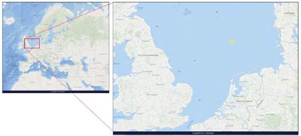
The main data of this study is a high-quality 3D PSTM from the F3 Block, located in the North Sea Offshore of Netherlands (Figure 2). Beside the seismic volume just mentioned the dataset contains geophysical logs, core and cuttings description for 6 wells (Figure 3). It is worth to mention that both the seismic survey and well information in the interval related to this study do not reveal any commercial discovery. Nevertheless, the dataset allowed to build a methodology that may be applied to an analog survey that shows similar geological features where it might be suitable for play definition and potential opportunities.
Petrophysics and Litho-types
The data processing started with the well log interpretation. Figure 4 shows the existing well log and sample (core and cuttings) description for one of the correlation wells.
The data shown in Figure 4 was used along with the implementation of techniques such as Linear Vshale estimation from Gamma Ray and neural net classification to get a 1D facies model that best described the stratigraphic column defined for the study area in the literature. Neural networks allow the interpreter to use as many well log properties as there are available to define clusters of points in a crossplot that best fit a certain rock type based on the physical properties given as input. Consequently, the clusters defined by applying neural network classification process represent specific rock types with a given range of each of the physical properties used as input. As a result of this process, the interpreter would differentiate a siltstone from a claystone, which is crucial when performing lithology estimation. Nevertheless, it is recommended to use stratigraphic columns created from the description of core and cuttings samples as input data to calibrate the interpretations of facies made from neural networks or any other methodology. Figure 5 illustrates a Crossplot where the ranges of the physical properties used as input can be observed for several of the defined facies.
In this context, using the ranges defined from the crossplots and the Vshale a 1D facies model was generated for all the correlation wells (Figure 6).
It is important to mention, that not all of the correlation wells have all the well logs required by the workflow here proposed (P-wave velocity, S-wave velocity, bulk density and total porosity) (Figure 3). Due to this lack of information, it was necessary to implement techniques to model the lacking physical properties. In particular, S-wave velocity is not available for all the correlation wells. To solve this issue, correlations between S-wave velocity and P-wave velocity such as the one proposed by Greenberg and Castagna (1992) (Figure 7) were implemented. After applying the Greenberg and Castagna (1992) correlations to estimate the S-wave velocity it was found that the elastic properties did not generate a sharp contrast between the facies interpreted in the correlation wells and so it was not going to be possible to run a lithology classification using just the elastic properties got by using the Greenberg and Castagna (1992) S-wave velocity model. Based on this fact, a new method for estimating S-wave velocity is proposed in this study where not only the P-wave velocity is used as an input but also the Vshale model is taken into account for estimating the S-wave velocity (Illidge, 2017). This method is based on the fact that both the S-wave velocity and P-wave velocity depend on the mineralogy of the matrix and so the more clay the slower both velocities would be. In this context, the correlation proposed by Illidge (2017) for estimating the S-wave velocity is given by equation 1.
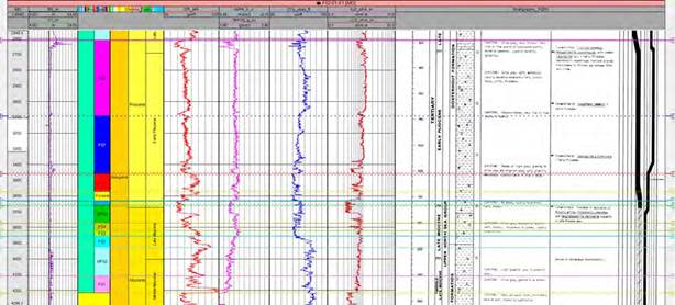
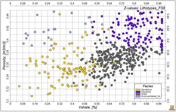
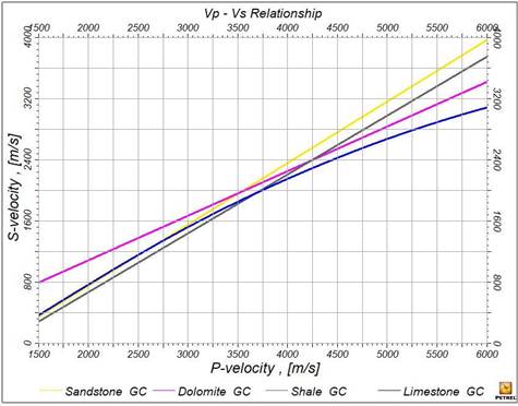
Figure 7 P-wave velocity to S-wave velocity correlations for different facies proposed by Greenberg and Castagna (1992).
 (1)
(1)
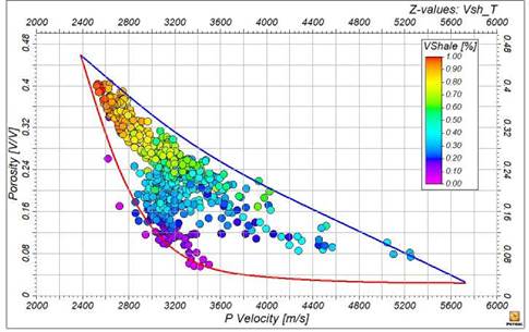
Where Vs corresponds to the S-wave velocity, Vp corresponds to the P-wave velocity and Vsh corresponds to the shale volume. It is worth to mention that this equation is not in the literature and therefore it represents a new approach in this process of physical properties modeling. For equation 1, the blue expression represents the trend for rocks with low or none shale volume while the red expression represents the trend for rocks with high shale content. Figure 8 illustrates an example made with data from the correlation wells where both limits, upper and lower, were defined from the interpretation of the point’s distribution. To have an idea of how well equation 1 predicts S-wave velocity, Figure 9 shows the resulting model of the application of equation 1 and its corresponding error estimated by comparing the modeled with the original S-wave velocity.
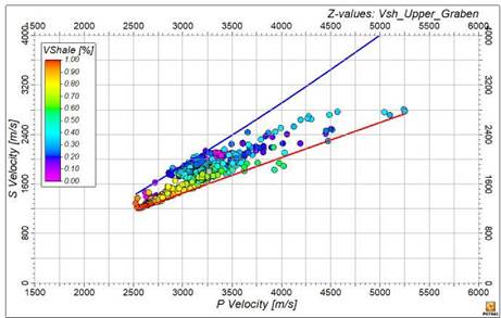
Figure 8 P-wave velocity vs S-wave velocity crossplot along with the limits defined to use equation 1.
Figure 9 S-wave velocity modeled (black curve in sixth track) by using equation 1 and its corresponding error (blue curve in seventh track) compared to the original S-wave velocity log (green curve in sixth track).
Using the same principle used to model the S-wave velocity, equations to model both the total porosity and the bulk density using as input the P-wave velocity and the shale volume for all the correlation wells in the interval of interest. In this context, equation 2 and 3 correspond to the expressions used to model the total porosity and bulk density where necessary.
 (2)
(2)
Where φ corresponds to the total porosity, Vp corresponds to the P-wave velocity and Vsh corresponds to the shale volume. It is worth to mention that this equation is not in the literature and therefore it represents a that this equation is not in the literature and therefore it represents a new approach in this process of physical properties modeling.
 (3)
(3)
Where ρ corresponds to the bulk density, Vp corresponds to the P-wave velocity and Vsh corresponds to the shale volume. It is worth to mention new approach in this process of physical properties modeling. Figure 10 and Figure 11 illustrate the corresponding crossplot and resulting model for each property.
Elastic properties
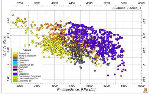
The main target of this process is to find the pair of elastic properties that shows the highest contrast between sandy and shaly facies. So, once all the required physical properties and the facies model were modeled the next step was estimating elastic properties such as P-impedance, S-impedance, Vp/ Vs ratio, Poisson’s ratio, Lambda and Mu. Now, with the elastic properties listed before a set of crossplots were made in order to find the crossplot to find the pair of elastic properties that shows the highest contrast between facies interpreted in the previous phase. These sort of crossplots are commonly named Rock Physic Templates (RPT’s) and are useful when it comes to running processes just like inversion feasibility (Lubbe and El Mardi, 2015). Figure 12 illustrates the RPT that best contrast the sandy facies from the shaly facies. Following the workflow from Figure 1, the last step of the 1D modeling is the elastic properties estimation and the selection of the best RPT for lithology estimation.
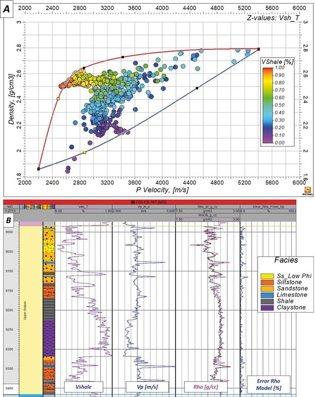
Figure 11 A. P-wave velocity vs bulk density crossplot together with the limits defined to use equation 3. B. Bulk density modeled (black curve in sixth track) by using equation 3 with its corresponding error (blue curve in seventh track) compared to the original bulk density log (magenta curve in sixth track).
Seismic-well tie
The first step in the 3D modeling corresponds to seismic-well tie and to perform the seismic-well tie analysis of the correlation wells the 1D models of P-wave velocity, bulk density as well as the well surveys and Formation tops of the interval of interest were used along with the 3D seismic data to get the final result, which is the time to depth relationship. This process was carried out in the software solution Hampson and Russell. The wavelet model to process the seismic-well tie was initially extracted in a statistical way from the seismic volume for the interval of interest and later a particular wavelet for each well was obtained as a result of the process. During the seismic-well tie process, any strong stretch or squeeze of the synthetic seismogram was avoid in order not to get resulting velocities that are not physically possible. In summary, a good correlation coefficient (greater than 0.5) was obtained for almost all of the correlation wells. Figure 13 illustrates an example for one of the correlation wells in which the correlation coefficient was 0.6.
Seismic interpretation (structural and stratigraphic)
Once the wells were tied to the 3D seismic information, a set of horizons corresponding to the interval of interest were interpreted. Figure 14 illustrates the geometry of the seismic volume used together with the correlation wells. Before starting the process of seismic interpretation, the PSTM image was conditioned following the workflow shown in Figure 15 to guarantee a better continuity of the reflectors during the interpretation of horizons and highlight the discontinuities for the application of geometric attributes. This process was carried out in the software solution Opendtect. To improve reflectors continuity, a guided dip filter was applied (Dip-steered Median Filter - DSMF) followed by a filter that highlights the reflector discontinuities (Fault Enhancement Filter - FEF). It should be noted that the seismic image used to calculate all the stratigraphic attributes corresponds to the DSMF model and the seismic image used to calculate all the geometric attributes was the one corresponding to the FEF model. Now, the first step in the seismic interpretation consisted in the interpretation of the main faults using as guide the seismic attribute of fault likelihood estimated in the software solution Opendtect.
After the interpretation of the main faults, the interpretation of the horizons corresponding to the members of the interval of interest was made in the software solution Petrel, generating a model of horizons and faults as shown in Figure 16. This set of horizons and faults were the input data for the generation of the 3D structural model of the interval of interest (Figure 17).
Once the structural model was built, the main horizons and faults interpreted on the conditioned seismic image were taken as a basis to generate a horizon framework with greater detail that follows all of the reflectors corresponding to the interval of interest one by one, honoring both the stratigraphic and structural features. In this context, Figure 18 illustrates the detailed horizon framework generated in Opendtect for Block F3. This horizon framework contains a total of 261 horizons that will allow greater detail in subsequent steps. The structural and stratigraphic model built for the entire interval of interest is well explained in Illidge et al. (2016). Based on the 3D horizon framework and the previously generated structural model, it was possible to generate a 3D model of seismic stratigraphy in which the main stratigraphic events associated with the interval of interest were interpreted. Figure 19 illustrates the stratigraphic model generated for Block F3. Thanks to the construction of this model of seismic stratigraphy it was possible to get some insights regarding the sedimentary environments associated to each of the levels found in the interval of interest, which in turn allowed to make a prediction of the possible lithologies expected for each member.
Figure 15 Seismic image conditioning workflow applied to improve reflector continuity and highlight discontinuities.
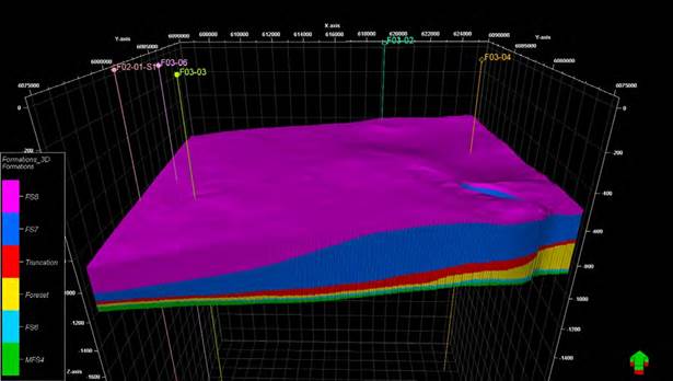
Figure 17 3D structural model generated from faults and horizons interpreted in the conditioned seismic volume.
Figure 18 Horizon framework built for the interval of interest honoring both structural and stratigraphic features.
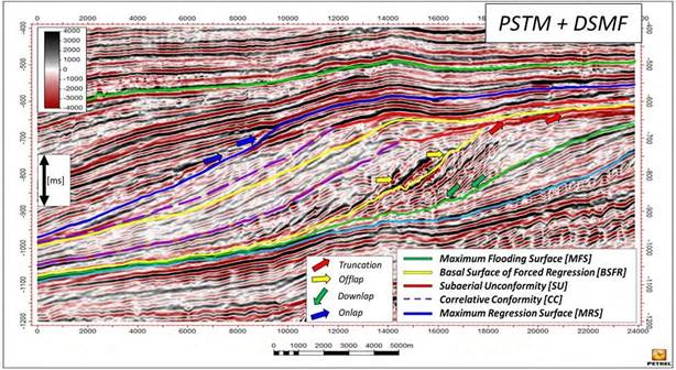
Figure 19 Seismic stratigraphic model built for the interval of interest. Taken from Illidge et al. (2016).
Attributes and seismic inversion
Before running the seismic inversion process, a set of seismic attributes were generated that were essential both for the seismic interpretation phase of faults, for which coherence attributes were used (Bahorich and Farmer, 1995), and horizons and for the properties propagation processes. Once the 1D modeling of the physical properties of the rock (Vs, Rho, Phi), seismic- well tie and seismic interpretation was done all the necessary information to perform the post-stacked seismic inversion of the seismic volume associated with the interval of interest was available. Now, the construction of the low frequency model was based on the horizon framework generated on a previous study (Illidge et al., 2016), which guarantees that the low frequency model honors both the stratigraphy and the structure of the interval of interest. Figure 20 illustrates a comparison between the conventional construction of a low frequency model using only the horizons found in Figure 16 and the construction of the low frequency model using the horizons found in Figure 18.
In this context, Figure 21 illustrates the acoustic impedance model obtained from the deterministic seismic inversion process performed in the software solution Opendtect. Likewise, Figure 22 illustrates the comparison between the acoustic impedance obtained from the inversion and the acoustic impedance estimated from well logs in which the good fit presented by the seismic inversion model can be seen.
3D properties propagation
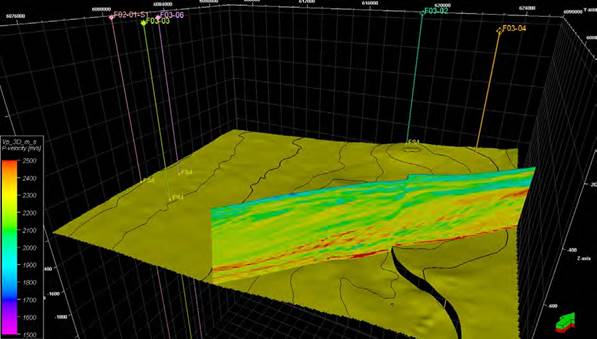
To get the 3D lithology model it is necessary to have 3D models of P-wave velocity, S-wave velocity and bulk density. To overcome this issue, it was necessary to use multivariate regression analysis between the acoustic impedance volume from seismic inversion, a list of seismic attributes and a specific target curve, so that at the end the input volumes could be converted to the missing physical properties just listed. This process was carried out on the software solution Hampson and Russell. The multivariate regression analysis method implements what is known as “Stepwise Linear Regression” to find the relationship between the seismic attributes and the target curve. Now, to estimate the P-wave velocity model, the information of the acoustic impedance and PSTM seismic volumes were initially extracted in the interval of interest over which a list of seismic attributes was run, which were filtered by their relationship with the target curve (P-wave velocity) thus generating a list of attributes in which the order is given by the relationship that this attribute presents with the target curve being the first attribute the one with the highest correlation coefficient. As it can be seen in Figure 23, initially the contribution of 20 seismic attributes were used to estimate the P-wave velocity model from which only 12 contributed to decrease the error between the estimated 3D P-wave velocity model and the profiles of this property in the correlation wells.
Figure 20 Comparison between low frequency models generated from 7 horizons (A. Conventional) and generated from 261 horizons (B. Sequence Stratigraphy).
Figure 21 Acoustic impedance model (B) generated by applying deterministic inversion to the seismic volume (A).
Figure 22 Comparison of the final acoustic impedance model obtained from deterministic seismic inversion (red) with the acoustic impedance model from well logs (blue) for two correlation wells.
Figure 23 Multivariable regression analysis between a list of seismic attributes and the P-wave velocity profile in the correlation wells.
As a result of this process, the 3D model of P-wave velocity is obtained for the interval of interest (Figure 24). The same workflow was applied to obtain the 3D models of S-wave velocity, bulk density and total porosity (Figure 25). Once the seismic attributes and acoustic impedance models have been integrated using multivariable linear regression analysis, it can be concluded that there is a strong correlation (in most cases non-linear) between the acoustic impedance and the estimated physical properties (P-wave velocity, S-wave velocity, bulk density and total porosity).
3D facies modeling
The 3D facies modeling phase was carried out in the software solution Hampson and Russell in which the main input data were the 1D models of facies and elastic properties generated in the correlation wells, the 3D models of elastic properties estimated from 3D models of P-wave velocity, S-wave velocity and bulk density and the horizons corresponding to the interval of interest. Now, based on the contrast presented by the ranges of P-impedance and VpVs ratio between sandy and shaly facies shown in Figure 12, this RPT was chosen for the 3D facies modeling. The first step in this workflow was the generation of probability distribution functions for each facies present in the interval of interest (Figure 26). These functions allow defining which facies is most likely to be present according to the range of elastic properties in which the data cloud is located. Further details about these probability functions can be found in Doyen (2007).
By applying these probability distribution functions on the 3D models of elastic properties it was possible to define the 3D facies model for the interval of interest. Figure 27 illustrates the 3D facies model which honors the defined sequence stratigraphic model in which the eastern region of interval of interest must have a higher content of sandstone and also follows the clinoforms associated with the delta analyzed.
Discussion
Implement seismic stratigraphy analysis as a qualitative parameter to control the results of 3D facies models have proven to be a key process in the generation of this kind of models.
Using a dense horizon framework for building the low frequency model represents a notable improvement in the quality of this variable, which has a great impact on the results of seismic inversion processes.
One of the main problems of the use of seismic inversion methods is the possibility of infinite solutions that satisfy the input data, which means that, for a particular seismic data there may be different geological models consistent with it and therefore it would be appropriate to implement stochastic methods to mitigate the uncertainty associated with these models.
Mainly, the seismic attributes that were not included in the estimation of the missing physical properties were either phase or wide window of analysis related, which did not contribute to the overall error for the missing physical properties estimation.
Integrate the largest number of reliable and useful information for the process (stratigraphic, structural, petrophysical and sedimentological models) may allow the interpreter to mitigate the uncertainty and improve the quality of subsurface models developed from seismic information.
Conclusions
As a result of this research, a new equation for the estimation of S-wave velocity taking into account parameters such as P-wave velocity and the volume of shale (Vshale) is proposed, which represents a contribution to knowledge in quantitative seismic interpretation.
The estimation of the S-wave velocity is a critical process in the quantitative seismic interpretation workflow, because it directly affects the estimation of elastic properties that work as input for facies classification or as hydrocarbon indicators in some rock types.
Multivariable analysis methods, such as the one implemented in this work, allow to define complex relationships between combinations of attributes and physical rock properties in an N-dimensional space (where N corresponds to the number of attributes used).
The use of elastic properties models integrated with geostatistical methods for data classification, such as the probability distribution functions, turns out to be appropriate in the generation of 3D facies model.

