


 Inglês (pdf)
 Artigo em XML
 Referências do artigo
 Enviar este artigo por email
 Citado por SciELO
  Citado por Google
  Similares em
SciELO
Similares em
SciELO  Similares em Google
 Permalink
Introduction
Ground Penetrating Radar (GPR) is a standard geophysical method used to identify shallow materials of the subsurface (<100 m). The GPR method is based on electromagnetic waves that are used to determine the properties of the soil, such as relative permittivity and conductivity. In general, the soil can be well characterized through relative permittivity and conductivity since they are indicators of the nature of the soil, moisture content, temperature, and the general geological structure. Those measures are also used to determine the texture of a surface layer because small particles of clay material increase the conductivity of the layer. Such characterization has relevance in applications such as ice analysis, mines and tunnels detection, pavement condition assessment and soil analysis for agriculture and, oil and gas exploration (Daniels, 2004).
In this case, the inverse problem consists of the determination or estimation of the profiles of relative permittivity and conductivity of the soil from data acquired at the surface. Recently, Full Waveform Inversion (FWI), has been used as a local optimization technique that allows estimating physical subsurface parameters from a set of observations at the surface. FWI has been applied in different contexts like seismic (Bunks et al., 1995), seismology (Blom et al., 2020), medical imaging (Guasch et al., 2020; Lucka et al., 2021), and electromagnetics (Lambot et al., 2004; Klotzsche et al., 2010; Mozaffari et al., 2020; Serrano et al., 2020).
The use of FWI with GPR data has many challenges, such as the initial model, the lack of sufficient illumination in the acquisition that produces high wavenumbers in the estimation of the parameters, the crosstalk between parameters, the high computational cost, and finally, the inverse problem is ill-conditioned and ill-posed. In this work, we propose a FWI method with two different regularizations that reduce the incoherent noise present in the data and produce a more stable solution. The proposed methods is tested in real GPR data collected in the municipality of Mogotes, Santander, in Colombia.
Theoretical framework
The Ground Penetrating Radar (GPR) is an electromagnetic method with applications in geophysics, civil engineering, and archeology (Daniels, 2004; Linde et al., 2010). The transmitter antenna emits an electromagnetic pulse into the soil, where the changes in the subsurface’s magnetic and electrical properties generate reflected, refracted, and transmitted energy. In a B-Scan acquisition, a set of consecutive radar waveform record along a particular direction, the energy is measured by one receiver antenna at some distance from the transmitter antenna. Figure 1A shows the principle of operation of a GPR system. Figure 1B shows the trajectories between the transmitter and receiver antennas using ray theory. The trajectories are air wave (AW); ground wave (GW); reflected wave (RW), and critically refracted wave (CRW). The AW trajectory is a direct wave, and its velocity is the speed of light in the air. The GW propagates slower than the AW, and it is a Surface wave. The RW is generated by the changes in the electromagnetic parameters of the subsurface (relative permittivity, relative permeability, or conductivity). According to Snell’s law, the CRW is generated at the critical angle.
Full waveform inversion
Full waveform inversion (FWI) is an iterative method that is being largely used to determine high-resolution models of the Earth’s subsurface from data acquired at the surface. The models of the soil are estimated by minimizing the difference between the recorded and modeled data. For the electromagnetic case, the relative permittivity εr(r), and conductivity models σr(r) can be estimated from the electromagnetic scan measured at the receiving antenna. The method starts at iteration k=0, with an initial model m0 for both parameters, and it is then updated iteratively by the method of Goldstein (1965).
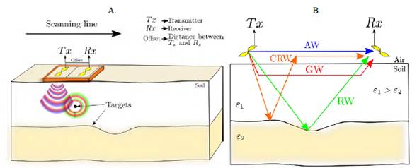
Figure 1 A. The principle of operation of a GPR system with two layers of contrasting permittivity (ε1 and ε2), modified from Persico (2014). B. Signal trajectories: air wave (AW), ground wave (GW), reflected wave (RW) and critical refracted wave (CRW); modified from Jol (2008).
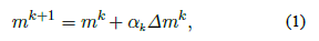
where αk is the step size and Δmk=-g(mk) is the gradient evaluated at mk. Each parameter is updated using the gradient function as follows
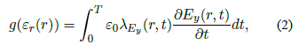
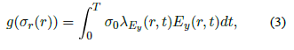
where Ey(r,t) is the electric field in the y-direction (V/m), ε0 is the permittivity in the vacuum and σ0 is a regularization value. Also, in Equations 2 and 3, λEy (r, t) is an adjoint field that simulates electromagnetic wave propagation but in reverse time. T is the final time of electromagnetic wave propagation.
Methodology
FWI with Gaussian function
The estimation of the electromagnetic soil parameters is proposed, in this work, via three different alternative cost functions for FWI. The first alternative cost function uses a Gaussian window. According to Xue et al. (2016), a smoothing parameter in the cost function allows for improving its convexity. FWI is a local optimization technique where the convexity of the cost function is desirable to avoid being trapped in local minima. The method proposed by Xue et al. (2016) uses a small number of misfit functions with smoothing kernels of decreasing strengths; during the FWI process, this allows the estimation of high-quality models with starting points that do not have enough low-frequency information. We have adapted the cost function to include the Gaussian function in the scansdirections, which is given by
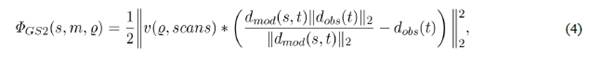
where ν (ϱ,scans) is a Gaussian function with standard deviation ϱ. The Gaussian function ν (ϱ,scans) is convolved with the difference between the modeled and observed data. The Gaussian function is defined as
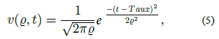
where  , t is the time vector, and T is the width of the Gaussian function. If the parameter ϱ2 is large, the cost function is not multimodal, which allows ignoring high-frequency information of the data. On the contrary, if the parameter ϱ2 is small, the cost function is multimodal, and the noise in the data together with an initial model without sufficient lowfrequency information produces a noisy solution. The Gaussian function helps converge to a solution of low wavenumbers that depend on the width of the window and the parameter ϱ.
FWI with Total Variation (TV) regularization
The second alternative for the cost function for FWI is the regularization of total variation (TV), used to reduce the noise contamination of the data (Rudin et al., 1992; Rodríguez, 2013). TV regularization seeks to obtain a smooth estimate while preserving the main structures. The cost function for FWI using TV regularization is given by Anagaw and Sacchi (2012).

where  and αTV is a small constant to avoid the numerical división by zero in the gradient.
FWI with Modified Total Variation (MTV) regularization
The modified total variation (MTV) is proposed by Lin and Huang (2014) as an alternative regularization method. The MTV regularization is a more stable version of TV since it does not depend on the  value included to avoid divisions by zero in the gradients. The MTV method is selected in B-scan acquisition as the first step to obtaining low wavenumbers in the image, which is difficult to obtain due to the lack of illumination during the acquisition. The MTV method is dictated by solving the following cost function
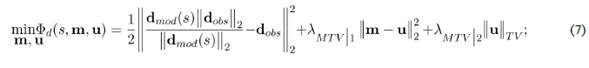
with
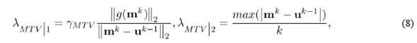
where γMTV can take values from 0.05 to 0.5 and k can take values from 0 to 200 according to Gao and Huang (2019). A large value of γMTV does not generate changes in the estimated parameters. On the other hand, a small value of the γMTV regularization results in the traditional FWI solution. Small values of k result in the traditional FWI solution, whereas a very high value for k results in a very smooth solution.
Experimental Results
Description of the experiment
The proposed methods are evaluated in the estimation of the electromagnetic soil parameters of a small area, located in Mogotes, a local municipality in the department of Santander, Colombia. The raw GPR data is acquired using a shielded antenna with a central frequency of 400 MHz. The acquisition line is shown in Figure 2A; it was selected near the Mogoticos river, where a visible outcrop is accessible. In the outcrop, two continuous geological layers of different rock materials are visible (Figure 2B). The acquisition includes 213 scans spaced 0.1 m. The total propagation time of the scan is 99.99 ns with 512 samples, and a time step of 0.195 ns. The acquisition line has a total length of 21.3 m.
Initial permittivity and conductivity
The first step to estimate the soil parameters is to determine an initial guess for the type of rock materials. For the area under study, only permittivity and conductivity were considered, and permeability is not taken into account. Picking the first wave arrival in the raw data is performed to find three significant reflectors, as shown in Figure 3. Then, the relative permittivity and conductivity values are selected taking into account the typical values of the subsurface materials and a visual inspection: in layer-A, the relative permittivity is 4, and conductivity is 1 mS/m, the material is considered a dry clayey soil. In layer-B, the relative permittivity is selected as dry-sand with a value equal to 6 and the conductivity is 1 mS/m; finally, the layer-C is chosen to be wet clay, and the relative permittivity value is 12 with conductivity of 4 mS/m.
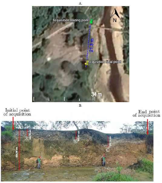
Figure 2 A. Acquisition line. B. Outcrop in the acquisition zone with three layers based on visual inspection: dry clay, dry sand, and wet clay soil, from top to bottom.
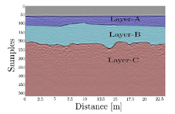
Figure 3 Raw GPR data interpretation with three continuous layers based on main reflectors: dry clay (layer-A), dry sand (layer-B) and wet clay (layer-C) soil.
The depth of each layer is obtained with the picking time and the relative permittivity of each layer. The first depth layer is computed using Equation 9 and the depths of the second and third layers are computed using Equation 10.
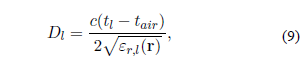
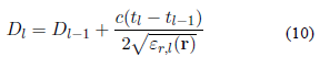
In Equations 9 and 10, l is the layer index, tl is the picking of the first wave arrival of the signal with higher amplitude, tair is the time for the air wave (approx. 0.9375 ns), is the velocity of electromagnetic waves in the vacuum, which is 3 × 10⁸ m/s, and εri,is the relative permittivity in layer l.
Figures 4A and 4C illustrate the permittivity and conductivity models for the layers. The spatial step of the images displayed in Figure 4 is 0.025 m in x- and z-directions. Figures 4B and 4D show the permittivity and conductivity models smoothed by a blurring filter of size 5 × 5.
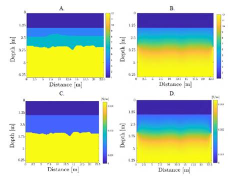
Figure 4 Initial guess for the electromagnetic parameters. A. Relative permittivity. B. Initial relative permittivity obtained after applying a smoothing filter on the model illustrated in Figure 4A. C. Conductivity. D. Initial conductivity obtained after applying a smoothing filter on the model illustrated in Figure 4C.
Source wavelet estimation using the impulse response In the GPR scenario of a B-scan acquisition, the antenna is located in the air, and the sign source can be estimated from the air-wave. The relationship of the source with the data in the air wave is linear; therefore, the observed data can be obtained as the convolution between the source (Js) and the impulse response of the earth (hearth).
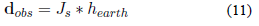
However, both the source and the impulse response of the earth are unknown. The impulse response of the earth can be estimated using a synthetic source and modeled data using the synthetic source (Belina et al., 2012). From the modeled and collected data, a background filter is used to select only the air wave, the details of this filter are presented in Khan and Al-Nuaimy (2010). The source is estimated from the observed data as

where IFFT is the Inverse Fourier Transform. According to Equation 12, the source can be estimated with a synthetic source with a sufficiently broad frequency bandwidth to avoid divisions by zero in the deconvolution, the modeled data, and the observed data.
The acquired raw data is shown in Figure 5A. However, to estimate the source signal, only the air-wave is needed, thus the direct arrivals are selected using an exponential time damping (Lavoué, 2014). The airwave of the acquired data is shown in Figure 5B. The source for the GPR system is obtained using the 213 scans and it is depicted in Figure 6, which shows the source in time and the amplitude spectrum of the estimated source signal. Also, the distance from the antenna to the surface was estimated to be 0.05 m.
Data preprocessing steps
The steps used in data preprocessing include the following:
Dewow filter: this filter selects a window and takes the mean value in the window to remove the DC components in each sample.
Lowpass filter (LP): FWI is a local optimization technique that begins with the estimation of the low frequency components of the parameters and then the high-frequency components. Since the data is collected using a 400 MHz antenna, the radargram has been filtered using a low pass filter at 250 MHz (Figure 7). Furthermore, the source is also filtered using the same corner frequences, which are depicted in Figure 8.
Background filter: The background filter is used to mitigate the horizontal and periodic events in the observed data, and it is called ringing noise. The ringing noise is removed using two steps, according to Khan and Al-Nuaimy (2010). The first step is to compute the eigenimages containing the highest and lowest values of the eigenvalues of the covariance matrix. The second step is to subtract the average value of the radargram. Figure 9B depicts the results when the background filter is applied to the data. The background filter is only applied in the first 500 samples where the air-wave is observed, and it avoids attenuation of some of the flat events that are of interest.
Resampling (optional): The time step required for numerical stability is obtained using the stability condition proposed by Courant-Friedrichs-Lewy (CFL). As the spatial step is Δh=0.025 m, we obtain that Δt⩽5.8966×10⁻¹¹ s. In compliance with this condition, the collected data is resampled to have a time step equal to 0.04 ns.
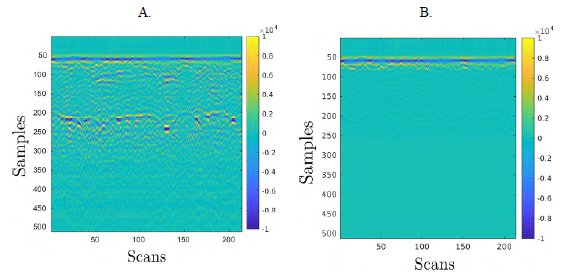
Figure 5 A. Acquired data. B. Observed data with an exponential time damping function to extract the air-wave only.
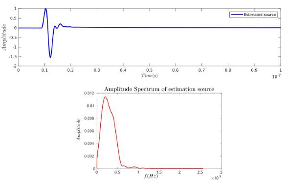
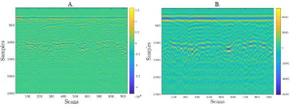
Figure 7 Collected data in the acquisition zone. A. Unfiltered data. B. Filtered data using a low pass filter between 0-250 MHz.
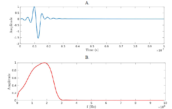
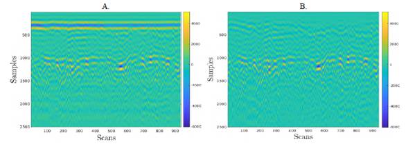
Figure 9 Background filter on the collected data. A. Data collected with low pass filter and without background filter. B. Collected data filtered with low pass filter and background filter.
FWI results using TV and MTV regularizations
TV and MTV regularizations allow for obtaining smoother solutions for the electromagnetic parameters in the inversion process. TV regularization has been included in the inversion process to analyze its behavior in the real collected data. Figure 10 shows the FWI results with TV regularization in both parameters (permittivity and conductivity). Different regularization values are tested in the experiment. Note in Figures 10B and 10G that having no regularization produces undesired values in the permittivity and conductivity parameters, which make no physical sense. In addition, to generate a smoother version of the parameters, the TV regularization does not allow extreme changes in the permittivity and conductivity values, so the inversion is more stable. Figures 10E and 10J present a very smooth solution for the conductivity parameter, so it is discarded. Similarly to TV regularization, MTV regularization is included in the inversion process. The regularization is tunned to 0.05. However, the parameter must be tuned. Figure 11B, Figure 11C and Figure 11D, show the inversion results with MTV regularization using the values κ(σ) = 100, 150 and 200, respectively. The MTV regularization converges to a less smooth model than the TV regularization. Both regularizations allow controlling the permittivity and conductivity parameters, preventing the conductivity from converging to undesired values.
FWI results with Gaussian TV and MTV regularization
TV and MTV regularization are combined in this section with the Gaussian window. The best estimation of the parameters is obtained using ϱ2 = 2 in scansdirections with a fixed window of length 66 using the FWI gradient resolution. The results of the TV regularization with a Gaussian function and the MTV with a Gaussian function are shown in Figure 12. The Gaussian window reduces the incoherent noise in the scans-direction and the solutions reach models with low-frequency information.
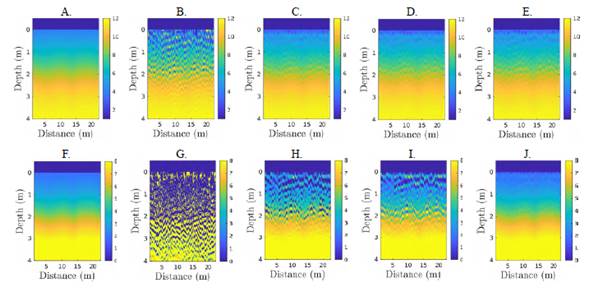
Figure 10 FWI with TV regularization, λTV (ε)=5.0×10⁻³ and λTV (σ) takes values of 2.5 x 10⁻³, 5.0 x 10⁻³ and 7.5 x 10⁻³. A. Initial relative permittivity. B. Relative permittivity no regularization. C. Relative permittivty and TV regularization λTV (ε)=5.0×10⁻³. D. Relative permittivty and TV regularization λTV (ε)=5.0×10⁻³. E. Relative permittivty and TV regularization λTV (ε)=5.0×10- 3. F. Initial relative conductivity. G. Relative conductivity no regularization. H. Relative conductivity and TV regularization λTV (ε)=2.5×10⁻³ I. Relative conductivity and TV regularization λTV (ε)=5.0×10⁻³ J. Relative conductivity and TV regularization λTV (ε)=7.5×10⁻³.
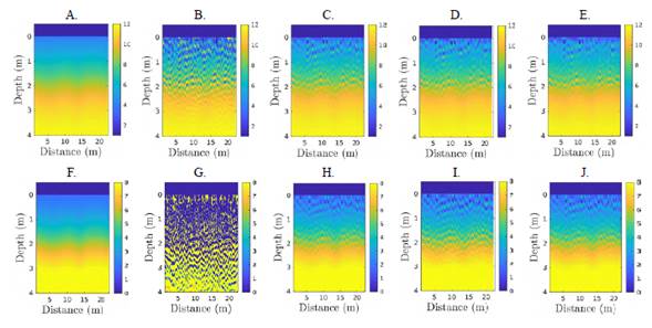
Figure 11 FWI with MTV regularization, κ takes values of 100, 150 and 200. A. Initial relative permittivity. B. Relative permittivity no regularization. C. Relative permittivty and MTV regularization κ =100. D. Relative permittivty and MTV regularization κ =150. E. Relative permittivty and MTV regularization κ =200. F. Initial relative conductivity. G. Relative conductivity no regularization. H. Relative conductivity and MTV regularization κ =100. I. Relative conductivity and MTV regularization κ =150. J. Relative conductivity and MTV regularization κ =200.

Figure 12 FWI with TV, TV+Gaussian, MTV and MTV+Gaussian. A. Initial relative permittivity. B. Relative permittivity no regularization. C. Relative permittivity and TV regularization. D. Relative permittivity and TV+Gaussian. E. Relative permittivity MTV regularization. F. Relative permittivity and MTV+Gaussian. G. Initial relative conductivity. H. Relative conductivity no regularization. I. Relative conductivity and TV regularization. J. Relative conductivity and TV+Gaussian. K. Relative conductivity MTV regularization. L. Relative conductivity and MTV+Gaussian.
Reflectiviy map of the FWI results
From the reflectivity map shown in Figure 13A and Figure 13B, the coherence of the horizontal events can be observed. The reflectivity map of the underground can be obtained using Reverse Time Migration (RTM). A Laplacian filter is applied to the imaging condition to remove the low-frequency artefacts due to backscattering in the RTM method, and a deconvolution is applied to the reflectivity map to remove the footprint of the source, such that the location of the reflector is detected. Two pairs of models of permittivity and conductivity have been used to obtain the reflectivity map: the FWI results models with the TV regularization using γTV(ε)=5.0×10⁻³ and γTV(σ)=5.0×10⁻³, and the FWI results models using the MTV regularization with κMTV=200. The results of each pair of models previously described are presented in Figure 13A and Figure 13B, respectively. Figure 13 shows that the reflectivity map for the MTV model is closer to the true solution than the reflectivity map obtained with the TV model.
TV and MTV regularizations search a smooth solution that preserves the main structures of the electromagnetic parameters. The results show that joining FWI with TV and MTV reaches a better estimation in the cost function and gives models with geological sense. The convexity in the cost function is promoted using TV and MTV regularization, it avoids being trapped in local minima with the high frequency information. However, the TV regularization is sensitive to high values in the gradient by the factor  . The results show a better estimation using MTV than TV for the conductivity values in the near-surface area, where better geologically constrained values are reached. The errors between the estimated reflectivity map and the real location of the reflectors, measured in the field, are: 1) in point A, 46 cm; 2) in point B, 14 cm and 3) in point C, 20 cm. TV and MTV regularizations, not only reduce the noise level but also preserve the primary interfaces. The experimental results show that the solution of FWI with regularization is not only smoother than traditional FWI but also the numerical result makes geological sense. Some areas of the traditional FWI solution indicate the presence of air, which is not geologically plausible.
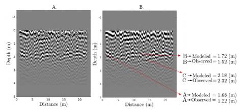
Figure 13 A. Reflectivity map for the TV models, and B. reflectivity map for the MTV models. Modeled and observed depths of points A, B and C (see Figure 2) are shown.
Summary and Conclusions
B-scan acquisitions are related to images of the subsurface that have high-frequencies. The limitation of the type of GPR system is that FWI requires an initial guess with enough low frequency information. By adding TV and MTV regularizations, the models of the electromagnetic parameters are smoother than using the typical FWI solution. Both regularizations, not only reduce the noise level but also preserve the primary interfaces.
The regularizations TV, MTV, and Gaussian window must have tuning stages of the regularization parameters such as γTV in TV, κ in MTV, or ϱ2 at Gaussian. These parameters can be obtained experimentally using several synthetic experiments. In this work, we have also provided a set of preprocessing steps that allows preparing the data for FWI.
The experimental results show that the solution of FWI with regularization is not only smoother than traditional FWI but also the numerical result makes geological sense. Some areas of the traditional FWI solution indicate the presence of air, which is not geologically plausible. We also found that by applying the Gaussian function in the scans-direction, the incoherent noise is reduced in the data while achieving a low-wavenumber solution of the model parameters

