




 Inglês (pdf)
 Artigo em XML
 Referências do artigo

 Tradução automática
 Enviar este artigo por email
 Citado por SciELO
 Citado por Google
 Similares em
SciELO
 Similares em Google

 Permalink


Introduction
For decades, the inversion problem has been a topic of great interest and impact in the field of computational geophysics. This makes it possible to infer the characteristics of a particular area by partially reconstructing the distribution of physical parameters obtained through geophysical exploration techniques (Tarantola, 2005; Isaev et al., 2022). Some of these parameters enable the inference of subsurface properties, including geological structure, magnetization, density, electrical resistivity, and electrical charge capacity (Reynolds, 2011; Sirota and Ivanov, 2018).
Resistivity is a measurement widely used in fields such as geotechnics, mining prospecting, hydrogeology, agriculture, and environmental sciences to gather and analyze information on subsoil's electrical properties related to composition, moisture content, salinity, and cohesion. Due to its applicability, methods have been developed in recent years for inverting data obtained by Electrical Resistivity Tomography (ERT). ERT is a non-destructive subsurface imaging technique that enables the detection of underground structures, water sources, and mineral deposits, as well as the conduct of geotechnical and environmental studies (Sjóberg et al., 2015; Berezowski et al., 2024). Resistivity data can be obtained at various resolutions and depths, depending on the electrode array, configuration, or matrix and the acquisition protocol used (Szalai and Szarka, 2008).
Some of the inversion methods used for ERT have been integrated into commercial software employing different approaches. For example, EarthImager™ 2D (Dastanboo et al., 2020; Alpaslan, 2021; Capa-Camacho et al., 2022; Zamanian et al., 2023) employs inversion algorithms such as penalized least squares, smooth modeling, and robust inversion based on the Gauss-Newton and quasi-Newton methods on either a block or triangular mesh (Redhaounia et al., 2015; Opatola et al., 2022; Advanced Geosciences, Inc., 2023).
Similarly, Res2Dinv (Arjwech et al., 2020; Aliou et al.,, 2022; Chibani et al., 2023) uses the fast least squares, damped least squares, and smooth-constrained least squares inversion algorithms modified based on the quasi-Newton, Marquardt-Occam (Marquardt method with constrained smoothness), and Gauss-Newton methods on either a block or unstructured mesh (Loke and Barker, 1996; Hellman et al., 2016; Loke et al., 2018; Zeynolabedin et al., 2021; Oliveira et al., 2023). AarhusInv (Mudler et al., 2019; Andersen et al., 2020; Genedi et al., 2021; Finn et al., 2022) utilizes the Laterally Constrained Inversion (LCI) and Spatially Constrained Inversion (SCI) algorithms based on the Gauss-Newton method with a Marquardt modification on either a block or triangular mesh (Auken and Christiansen, 2004; Auken et al., 2015; Lin et al., 2019).
Finally, ZondRes2D (Idfi et al., 2019; Kukemilks and Wagner, 2021) features the regularized least squares inversion algorithm based on the Gauss-Newton, incomplete Gauss-Newton, and nonlinear conjugate gradient methods on a block mesh (Zond Software, 2022). Additionally, to calculate resistivity values, these tools typically employ the finite difference method for data collected in regions with flat layers, and finite elements for data collected in regions with more complex topographies (Loke et al., 2018). Moreover, these inversion methods are used in some open-source environments based on C++ and Python, including BERT, pyGIMLi, pyres, ResIPy, and SimPEG (Doyoro et al., 2022). These packages emerge as an alternative solution to some of the drawbacks found in commercial software, such as the inability to filter out current and potential electrode noise, remove outliers, and modify resistivity maps by manipulating ERT data. Such drawbacks require the use of additional computational tools (e.g., x2ipi and Prosys), self-created routines, among other strategies (Placencia-Gómez et al., 2010; Bingham and Legault, 2018; Azaiez et al., 2020; Porras et al., 2022; Yonli et al., 2023).
Regarding inversion results, while Res2Dinv is fast and efficient, it struggles to adapt to non-rectangular topographies, resulting in vertical expansion in the generated data. Conversely, while AarhusInv is algorithmically more complex and slower than Res2Dinv, it adapts better to complex topographies. However, it also tends to produce horizontalexpansions. PyGIMLi falls somewhere between Res2Dinv and AarhusInv in terms of speed and adaptability. Nonetheless, it is not effective in solving structures with sharp geometries, leading to rounded anomalies. This problem can be minimized by properly adjusting the regularization parameter 1 in the pre-weighted Gauss-Newton scheme, which is iteratively employed with ridge regularization (Tikhonov regularization) (Hellman et al., 2016; Rücker et al., 2017; Von Bülow et al., 2021; Jabrane et al.,, 2023). One of the challenges in employing Tikhonov regularization in models or schemes like pyGIMLi is finding the most efficient approach for solving this inverse problem considering that the parameters obtained from geophysical exploration are non-linear. The regularization parameter 1, which controls the balance between data fidelity and prior information, allows us to reach the solution to the inverse problem that is more suited to its characteristics and correct the rounded anomalies found in the framework (Oraintara et al., 2000). Different methods have been developed to estimate this parameter, including maximum likelihood (ML), ordinary cross-validation (OCV), generalized cross-validation (GCV), the discrepancy principle (DP) (Morozov, 1984; Okamoto and Li, 2007), the L-curve (Quiceno et al., 2022), and genetic algorithms (GA) (Wu et al., 2008; Zheng et al., 2019). Since pyGIMLi lacks a function or class to estimate the optimal 1 value, it is common practice to use trial-and-error methodologies to find it. For example, Quiceno et al. (2022) developed an algorithm based on the L-curve in conjunction with a curvature function to semi-automatically estimate it.
The discrepancy principle (DP) selects the regularization parameter by enforcing that the residual norm of the reconstructed solution remains commensurate with the estimated noise or error level in the data. In essence, it constrains the solution to remain within the fidelity limits imposed by the data quality, thus mitigating overfitting and underfitting. Originally formulated by Morozov (1984) , building upon foundational work dating back to the 1960s, the DP has become a well-established and rigorous criterion within the broader framework of Tikhonov regularization for addressing ill-posed inverse problems in which noise may strongly influence the solution.
In contrast to the DP, methods such as maximum likelihood (ML), cross-validation (CV), and generalized cross-validation (GCV) rely explicitly on statistical assumptions regarding noise characteristics and data structure. Other strategies, such as the L-curve method or genetic algorithms (GA), tend to introduce a higher degree of subjective interpretation, particularly under conditions of severe noise or strong ill-posedness, as is commonly encountered in electrical resistivity tomography (ERT). In such contexts, the DP offers an intuitive and model-agnostic criterion whose reduced dependence on specific probabilistic assumptions facilitates its practical adoption and enhances confidence in the stability of the resulting solutions.
This paper describes the implementation and validation of a consecutive approximation algorithm based on the discrepancy principle to automatically estimate the optimal λ value in the pre-weighted Gauss-Newton inversion scheme.
The algorithm was validated using three datasets from different sources and characteristics to thoroughly test its effectiveness in various contexts and applications. The first dataset is a synthetic mixed anomaly model in homogeneous layers taken from an example in the pyGIMLi library. The second dataset corresponds to a replicated synthetic model of conductive blocks. Lastly, the third dataset is a slag dump profile, which is also available as an example in the same library but was originally described and employed in 2006.
Materials and methods
Gauss-Newton scheme and discrepancy principle Tikhonov regularization is a widely used method for solving ill-conditioned problems by introducing a regularization term that modifies the objective function of a system (Sirota and Ivanov, 2018). Equation 1 shows a general expression that describes the operation of Tikhonov regularization, where ϕ d is generally a measure of the error between the model predictions and the actual data, known as the residual norm. For its part, ϕ m is a regularization term that imposes constraints such as L1 or L2, where a sum of absolute values or the square root of the sum of squares is applied to the possible values of ϕm, so it is known as the solution norm (Tikhonov, 1963, 1966; Willoughby, 1979; Tikhonov et al., 1995).
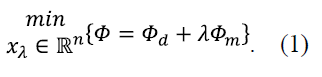
The regularization parameter 1 is the value that controls the balance between data fidelity and prior information. In other words, it maintains the balance between the ϕ d and ϕ m norms, and hence the result of the objective function that requires to be minimized. This concept is crucial in the pre-weighted Gauss-Newton scheme used in pyGIMLi and shown in equation (2):

where 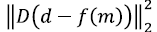 is the residual norm and
 is the solution norm. Here, D is the diagonal matrix of the relative error; d is the logarithmic apparent resistivity vector; m is the logarithmic resistance vector; f(m) is the response model of m; and C corresponds to the identity if m
0
is a model with a priori information, or serves as a feature control of the scheme if m
0
is a constant vector (Rücker, 2011; Quiceno-Arenas et al., 2022).
The discrepancy principle will be used to select λ. According to this principle, λ can be chosen when the following equality is achieved:
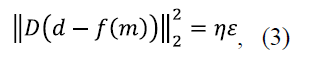
where ɳ is the tolerance value (preferably >1) and Ԑ is the error size (Sizikov and Sidorov, 2017; Schenkels and Vanroose, 2018). In the case of Gauss-Newton methods, where the dataset covariance is known, as in the pyGIMLi inversion scheme, the error size is proportional to the N data size (Günther, 2004; Petra et al., 2012). Therefore, a value ɳ = 1 is expected to lead to a residual norm equal to the data size:

Thus, the optimal λ value is obtained by satisfying equation (4).
Dataseis
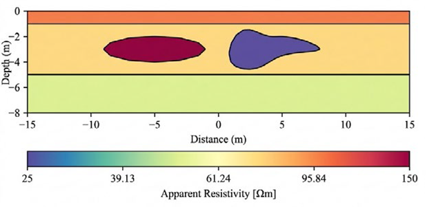
Mixed anomaly model in homogeneous layers: This dataset corresponds to a synthetic model that features mixed anomalies and is characterized by a flat topography with three homogeneous layers, each with defined apparent resistivity data. The second layer includes a uniform and a non-uniform structure as anomalies, which also have a defined apparent resistivity value (Figure 1) (pyGIMLi, 2023a). Resistivity data were collected using a Dipole-Dipole electrode array with a spacing of 1.5 meters, a Gaussian noise of 1%, and a voltage error of approximately 1 V.
Conductive block model: This model features a length of 16.2 meters and a depth of 5.4 meters. It has a flat topography and contains two conductive blocks of 2.5 meters in length and 0.3 meters in height (Figure 2) (Zamanian et al., 2023). The ResIP framework was used to perform the modeling, employing Dipole-Dipole, Wenner a, Schlumberger, and Multi-gradient electrode arrays with a spacing of 0.6 meters and a Gaussian noise of 2%. Figure 2A shows the synthetic model created in pyGIMLi, where Region 1 (50 Ωm) represents the background layer and Region 2 (5 Ωm) and Region 3 (10 Ωm), the conductive blocks.
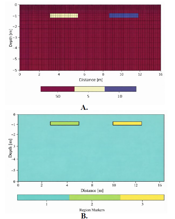
Figure 2 Synthetic conductive block model. A. Adapted from Zamanian et al. (2023) and B. created in pyGIMLi.
Real slag dump data: This dataset corresponds to a slag dump from steel production, which features a width of 70 meters and a maximum height of 14 meters above ground level. A total of 222 data points were collected using a Wenner a electrode array with a spacing of 2 meters (Günther et al., 2006). At its electrodes, the minimum and maximum elevation recorded was 108.45 meters and 121.20 meters, respectively (pyGIMLi, 2023b). Figure 3 displays the distribution of the samples taken using pseudosections from the electrode array and spacing along with the apparent resistivity values (Figure 3A) and topographic effect values for such data (Figure 3B). The topographic effect values were obtained by computing the ratio between the numerically calculated geometric factor that accounts for topography and the analytical formula that does not.
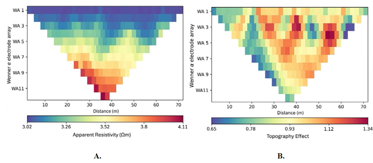
Figure 3 Pseudosections from electrode array and spacing of the A. apparent resistivity values and B. topographic effect (pyGIMLi, 2023b). WA refers to Wenner a, and the value next to it to the electrode spacing applied in the data acquisition protocol.
Consecutive approximation algorithm and inversion parameters
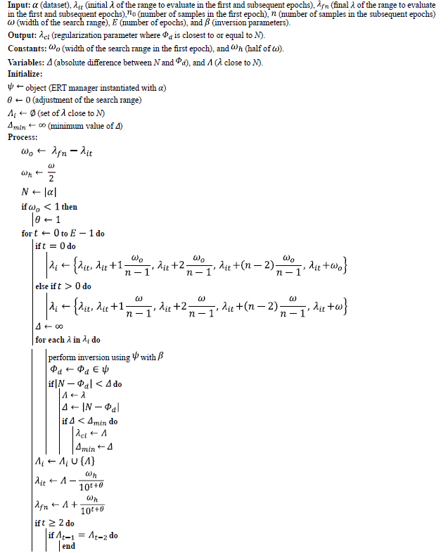
The pseudocode shown in Algorithm 1 describes the process for estimating the optimal λ value for arbitrary datasets that depend on solving the inverse problem. Given that the ERT inversion manager in pyGIMLi allows the value of ϕ d to be estimated for an inversion with specific parameters, an iterative process must be carried out for the various ranges of λ that are evaluated. Also, another iterative process must be performed to evaluate each value of that range to arrive at the approximation that is most consistent with the ideal value. Since the algorithm makes it possible to assign an initial range for λ, as well as an initial number of samples and the number of epochs to be run, the proposed approach may adapt to the different datasets that can be processed. The inversion parameters (i.e., the inversion characteristics of the scheme) included the maximum cell size of the unstructured mesh (paraMaxCellSize) and the boundary extrapolation (paraBoundary). Moreover, it is worth noting that n is the output parameter of X 2 in pyGIMLi.
Results and discussion
The results section provides a comprehensive validation of the consecutive approximation algorithm (Algorithm 1), which was designed to automatically determine the optimal regularization parameter (λ 0) within the pre-weighted Gauss-Newton inversion scheme. The primary objective of the validation was to demonstrate that the algorithm could robustly converge on a λ value that satisfies the discrepancy principle, resulting in an ideal tolerance value (X2 «1.00) across various data scenarios. This target X2 value signifies that the error between the model and the data aligns perfectly with the data size, indicating a highly accurate and ideal fit.
The algorithm's performance was assessed using two synthetic Electrical Resistivity Tomography (ERT) models-one with a mixed anomaly in homogeneous layers and another with a conductive block-as well as a real-world slag dump profile. In all tests, the proposed method successfully converged to the optimal 1 within a limited number of epochs, consistently yielding inversion models with X 2 values precisely at or near 1.00. Furthermore, a comparative analysis against an L-curve-based approach (Algorithm 2) revealed that the proposed Algorithm 1 offers superior automation, greater self-sufficiency, and enhanced computational efficiency. Crucially, the resulting inversion models, particularly those for the synthetic conductive block, demonstrated improved subsurface structure definition and better handling of background layer distribution, showcasing its practical advantage over other established inversion frameworks.
Figure 4 presents the approximation results for the estimation of λ in the synthetic mixed anomaly model in homogeneous layers using the proposed method. As shown in Figure 4C, the optimal value was found at epoch 5. Figure 5 shows the response model obtained with the optimal regularization parameter (λ 0), where the ideal tolerance value (X 2 =1) was achieved.
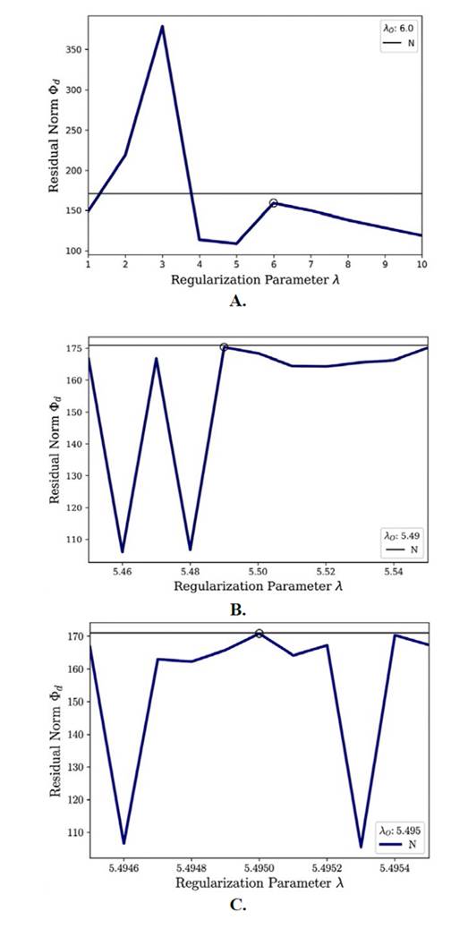
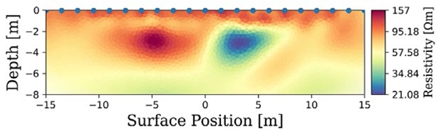
Figure 5 Unstructured mesh response model (ERT) in the synthetic mixed anomaly model in homogeneous layers with λ0= 5.4746, using the consecutive approximation algorithm.
Figure 6 displays the optimized response model in the mixed anomaly model in homogeneous layers (Figure 1). It was obtained using an algorithm that combines the L-curve and a curvature function (see Algorithm 2) to estimate the optimal regularization parameter (Quiceno et al., 2022).
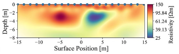
Figure 6 Unstructured mesh response model (ERT) in the synthetic mixed anomaly model in homogeneous layers with L-curve. From Quiceno et al. (2022) .
In the case of the slag dump, Figure 7 shows the approximation results for the estimation of 1O using the proposed method. The optimal value was achieved at epoch 5 (see Figure 7C). Furthermore, Figure 8 displays the response model obtained with the estimated 1O value, where, as expected, an ideal tolerance value was achieved.
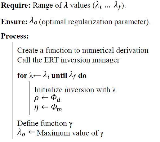
Note: Adapted from Quiceno et al. (2022) .
Algorithm 2 Selection of the regularization parameter in pyGIMLi using the L-curve method.
There is a high correlation between the data processed in both the response model obtained with the L-curve method and the response model obtained with the discrepancy principle. The anomalies introduced in the modeling process, along with a significant portion of the homogeneous layer distribution, can be differentiated. However, it is worth noting that the inversion parameters were not the same when the two proposed algorithms were validated.
When the results of Algorithm 2 (L-curve method) were compared with those of Algorithm 1 (consecutive approximation), the latter was found to be significantly more automated and self-sufficient because it can easily adapt to more flexible or critical search regions that change gradually with each epoch. This simplifies the learning curve and application of the proposed algorithm for the final user, making it considerably more useful and less laborious. Finally, by avoiding the repetitiveness of λ O and successfully managing to automatically adapt to the number of samples n in the successive search regions, Algorithm 1 significantly outperformed Algorithm 2 in terms of the computational resource and time required to obtain the best regularization parameter.
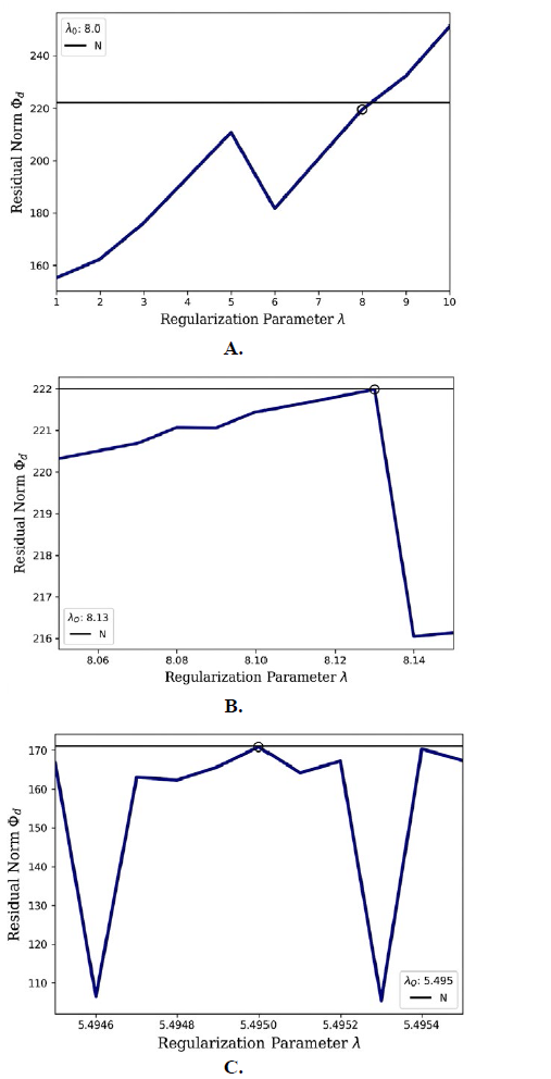
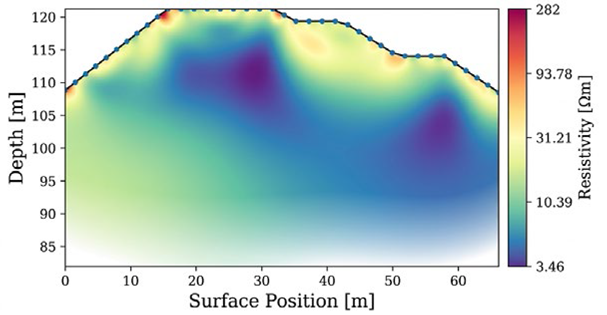
Table 1 contains the optimization process parameters used in the mixed anomaly model in homogeneous layers and the slag dump profile.
Table 1 Optimization and inversion process parameters of the mixed anomaly model in homogeneous layers and the slag dump profile.
| Dataset | Algorithm | Inversion | Output | |||||||
|---|---|---|---|---|---|---|---|---|---|---|
| λ i | λ f | ɳ | E | MaxCell | Boundary | λO | E0 (b) | Χ2 | RRMS(c) (%) | |
| MAMHL(a) | 1 | 10 | 10 | 5 | 0.1 | 0 | 5.4746 | 5 | 1 | 1.00 |
| Slag dump | 8.1315 | 3.00 | ||||||||
( a)MAMHL = mixed anomaly model in homogeneous layers. (b)RRMS = relative root mean square. (c)It represents the epoch where the optimal 1 value was found.
Finally, Figure 9 shows the approximation results for the estimation of λ in the conductive block model. The D-curves for the first iteration are shown in the left column, and the D-curves for the optimal λ value are shown in the right column. Figures 9A, 9B, 9C and 9D correspond to the Dipole-Dipole, Wenner α, Schlumberger, and Multi-gradient electrode arrays
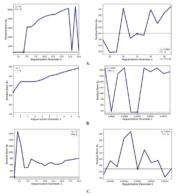
Figure 9 Discrepancy curves (D-curves) of the initial and final epochs for the optimal λ value in the four electrode arrays employed in the conductive block model. A. Dipole-Dipole, B. Wenner, C. Schlumberger and D. Multi-gradient.
Table 2 contains the technical information gathered from the conductive block modeling with the different electrode arrays. Each dataset showed an absolute relative error of 2%, which indicates clean Gaussian noise in the modeling process when using a voltage error of approximately 0.1 V.
Table 2 Technical information of the conductive block model datasets.
| Array | N(a) | Error(b) | |
|---|---|---|---|
| Min (%) | Max (%) | ||
| Dipole-Dipole | 325 | 2 | 2 | __ _
| Wenner | 117 | ||
| Schlumberger | 169 | ||
| Multi-gradient | 140 | ||
( a)Amount of data obtained with the pyGIMLi modeling protocol for each array. (b)Relative error of the dataset.
Table 3 lists both the parameters used in Algorithm 1 and the parameters obtained from the inversion with the λ O value found.
Table 3 Optimization and inversion process parameters of the conductive block model datasets.
| Array | Algorithm | Inversion | Output | |||||||
|---|---|---|---|---|---|---|---|---|---|---|
| λ i | λ f | n | E | MaxCellSize | Boundary | λO | E0 (a) | Χ2 | RRMS(b) (%) | |
| Dipole-Dipole | 0 | 4.496003 | 8 | 1 | 1.00 | |||||
| Wenner a | 1 | 20 | 20 | 10 | 0.005 | 1.0381 | 6 | 2.24 | 2.90 | |
| Schlumberger | 0.9505 | 6 | 0.99 | 1.98 | ||||||
| Multi-gradient | 1 | 10 | 10 | 10 | 0.01 | 1.0394 | 5 | 0.82 | 1.80 | |
( a)RRMS = relative root mean square. (b)It represents the epoch where the optimal λ value was found.
After comparing the relative error of the dataset and the relative error obtained from the inversion with λ0, and after analyzing the relative error obtained for the first two datasets (Table 1), we observe that the response model fits the absolute relative error (i.e., the error size ) by obtaining an ideal tolerance value (or a value close to it). This indicates an ideal fit between the response model and the dataset, in contrast to obtaining a relative error better than the induced Gaussian noise, as is the case of Zamanian et al. (2023) , with a RRMS lower than 1.2% in their response models.
In Figure 10, the response models obtained in ResIP (Zamanian et al., 2023) are displayed in the left column and those optimized with pyGIMLi, in the right column. Figures 10A, 10B, 10C, and 10D correspond to the Dipole-Dipole, Wenner α, Schlumberger, and Multi- gradient electrode arrays, respectively.
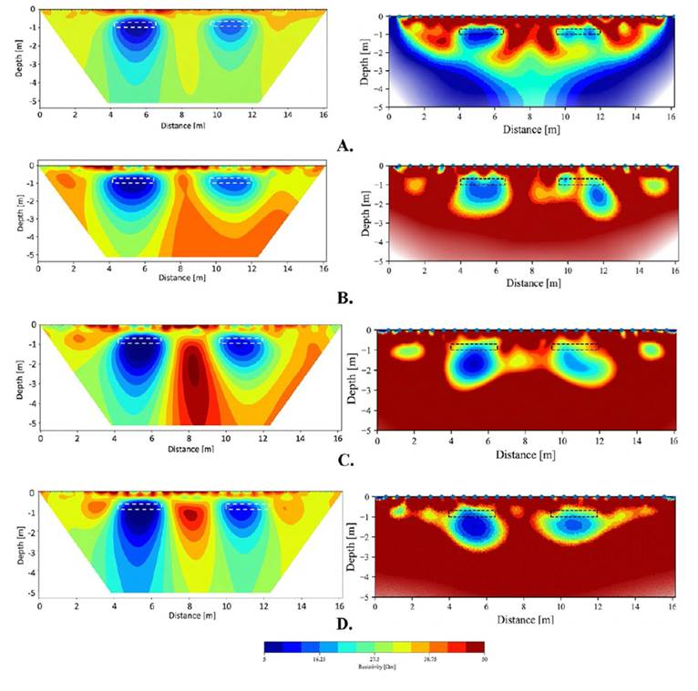
Figure 10 Response models (ERT) with ResIP and pyGIMLi (with ) for the four electrode arrays employed in the conductive block model. A. Dipole-Dipole. B. Wenner . C. Schlumberger. D. Multi-gradient.
When compared to each response model, the proposed algorithm demonstrates an improved distribution of the background layer and reduced vertical expansion of the conductive blocks. This improvement is attributed to better control of the rounded anomaly resulting from the optimal regularization parameter. However, a vertical displacement with respect to the original positions of the conductor blocks has been observed, which could be attributable to the configuration of each array. Particularly, the Dipole-Dipole array stands out for having good vertical resolution and considerable depth of investigation. Conversely, the Wenner a, Schlumberger, and Multi-gradient arrays, while displaying good horizontal and lateral resolution, do not achieve comparable depth of investigation (Szalai et al., 2009; Loke et al., 2018). Table 4 shows the comparison between the different arrangements.
Table 4 Comparison between the different arrangements.
| Array | Dominant sensitivity | Depth of investigation | Inversion resolution |
|---|---|---|---|
| Dipolo-Dipolo | Lateral: High | High | High |
| Wenner-α | Vertical: High | Moderate | Low/Medium |
| Schlumberger | Mixed: Moderate | Medium/High | Medium |
| Multigradiente | Mixed: High | High | Very High |
Regarding the obtained E O , it is important to consider that the optimal regularization parameter may not always be achieved in the final epoch. This is because there may be even closer proximity to N in the initial or intermediate iterations, as seen in the conductive block model. Therefore, Algorithm 1 considers this selection criterion to deliver the optimal regularization parameter.
Furthermore, prior knowledge of the data (e.g., number of samples) is crucial to define the initial search region (range of 1 values) that best fits the difference between the theoretical and generated or observed values (Wang et al., 2010). Nonetheless, choosing a search region smaller or larger than 1 does not affect the functionality of the consecutive approximation algorithm, as it has built-in compensation for the designated search region during implementation.
Conclusions
The consecutive approximation algorithm proposed in this study enabled us to estimate the optimal regularization parameter for solving the inverse problem using the Gauss-Newton scheme and ERT data.
The proposed algorithm was validated using both synthetic and real data and compared with another algorithm based on the L-curve method (see Algortithm 2) (Quiceno et al., 2022). According to the results, the proposed algorithm was able to estimate an optimal value for the regularization parameter Q.), with good correlation between the observed and theoretical data, as well as an ideal tolerance (X2) for both datasets.
Although the response models of the two algorithms (i.e., the L-curve algorithm and the one proposed in this study) exhibit similarities in the obtained images, the proposed consecutive approximation algorithm proved to be more efficient and flexible. This is because the regularization parameter estimation no longer involves previously assigned search intervals or trial-and-error testing. These advantages make the proposed algorithm -based on the discrepancy principle- a promising tool for geophysical data inversion, as it can adapt to different datasets, numbers of measurements, and search regions, facilitating its use in a variety of scenarios. Considering this, the results of this study contribute to enhancing the processing and interpretation of ERT data and provide a foundation for future research on related methods or applications.

