


Services on Demand
Journal
Article
 English (pdf)
 Article in xml format
 Article references
 Send this article by e-mail
Indicators
-
 Cited by SciELO
 -
 Access statistics
Related links
-
 Cited by Google
 -
 Similars in
SciELO
Similars in
SciELO -
 Similars in Google
Share

 Permalink
Revista Colombiana de Ciencias Pecuarias
Print version ISSN 0120-0690On-line version ISSN 2256-2958
Rev Colom Cienc Pecua vol.18 no.1 Medellín Jan./Apr. 2005
SELECCIONES
Origin and comprehensive study of Thünen´s model to analyze data from in situ rumen degradability technique
Héctor J Correa, MSc1.
1Assistant Professor. National University of Colombia, Medellín Campus. Animal Production Department.
(Recibido: 23 marzo, 2004 ; aceptado: 14 diciembre, 2004)
Summary
The classical model utilized to analyze data from in situ rumen degradability technique was originally proposed by Thünen to study the harvests responses to different production factors. In order to settle the meaning of kd in the Thünen´s model, a mathematical analysis was realized which indicated that this constant represents the quotient between the ruminal degradation acceleration and velocity. Similarly, the kp constant represents the quotient between the ruminal passage acceleration and velocity.
Key words: degradation acceleration, degradation velocity, derivation, exponential models
Introduction
Although the in situ degradation technique is one of the most frequently used in food evaluation to ruminants, it has been recognized that its results depend on several methodologic factors (17). The mathematical model used to estimate the parameters of ruminal kinetics from data of in situ degradation, also can affects the results and can explains the lack of response to supplementation with nutritional undegradable fractions in rumen (3). Other reason in the absence of response is the interpretation of the results and its application to the estimation of the degradable and non degradable fractions in the rumen.
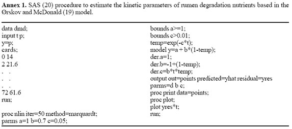
Since 1970, when Waldo (25) proposed a mathematical model to the analysis of data from in situ ruminal degradability technique, it has been published several alternative models to try to improve their prediction capacity and the understanding of this process (11, 13). One of this models was the one proposed by Ørskov and McDonald (19). It had beenconverted in one of the most frequently used to the study of ruminal degradation kinetic and it had been incorporated as the reference model in several systems to food protein evaluation to ruminants (1, 16, 21) (see in Annex 1 the SAS (20) procedure to estimate the kinetic parameters). Nevertheless its popularity, the interpretation of one of the terms of the model is still unclear and it had determined, in consequence, the erroneous
interpretation of the results. This confusion is possibly due to this model was originally developed to other purposes and due to the ignorance of the mathematical and kinematical interpretation of it. The objectives of this paper were to review the origin of the model proposed by Ørskov and McDonald (19) and to discuss the mathematical interpretation of each terms and the complete model.
The model origin
Ørskov and McDonald (19) proposed the non lineal exponential model y = a + b(1-exp(-kd t))A*,for the analysis of the data obtained trough the in situ ruminal degradability technique, being the most used model for this purpose (11, 15, 16). Although this model had been credited to this authors (12, 18), this was known before as Mitscherilch´s model (14) because this researcher was who utilized it for the study of the responses of harvest to different fertilizing dose named it as “law of the soil”. This law was mathematically represented by this author as dP/dF = k(B -P) B*, which represents the marginal productivity of fertilizer (dP/dF) as a constant fraction of the difference between the maximum (B) and real level (P) of production. After integrating this equation, it is obtained (8) P = f (F) = B(1 -e-kF) C*.
Spillman (22), in an independent paper, obtained the same Mitschelich´s equation calling his model as “law of the diminishing increment”.
Neither of this authors, however, were aware that before the German agronomist and economist Johann Heinrich von Thünen (24), had been developed a similar model in an effort to identify empiricaly the production relationship in his farm. To solve this problem, Thünen, applied the marginal analysis to all production factors and prices (8).
The experiments done by Thünen in Mecklenburg (Germany), suggested to him that the successive increases of any production factor - keeping constant the others -caussed that the production is increased in a constant fraction related to the amount added by the preceding unit. This fraction was two-thirds for labor, nine-tenths for capital and one-half for fertilizer (8).
Accepting that the fractional relationship between the marginal products obtained for any variable production factor can be denoted as r, the increased factor in the incomes constitutes the diminishing term of the geometric series a, ar, ar2, ar3, . . . arn-1, where a is the marginal product of the first unit of the factor, ar the marginal product of the second unit, ar2 the marginal product of the third and so until it is reached the last unit, nth, whose marginal product is arn-1 (8).
Using the formula to the sum series it is obtained S = [a(1 -rn)/(1 -r)] D*. The sum of the n marginal products gives the factor’s total product as P = B(1 -rn) E*, where B denotes the constant term a/(1 -r) and the exponent n is the number of units of the variable factor utilized. Due that r is a fraction such that rn trends to zero when n becomes infinite, it is deduced that B is the limit that the sum B(1-rn) approaches as the number of factor units n that becomes infinitely large. The last result obtained is that the total sum converge asymptotically with the maximum B value (8).
The same analysis is held to others variable production factors. In consequence, when it is allowed that all factors vary simultaneously, the production function that underlyies Thünen´s experiments can be expressed as P = f (L, C, F) = B(1 - 2/3L)(1 - 9/ 10C)(1 - 1/2F) F*, where the exponents denote the amounts utilized by each factor. This apply when factors vary in discrete units. When this units are infinitely divisible and continuously variable, then the term e -k replaces the factor r in the production function. In this case, k denotes the instantaneous rate of decreasing in the marginal productivity and e-k is the factor of proportionality over the unit interval. The result obtained is that the total product of each factor becomes as P = B(1 -e-kn) G*. This function, like its discrete counterpart, possesses two properties: first, the output is zero when any factor is zero and second, the output approaches its maximum level B when all factors are increased indefinitely (8).
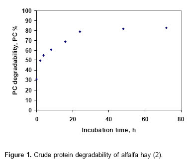
Mathematical interpretation of Thünen’s model for the analysis of data from in situ ruminal degradability techniqueData from in situ ruminal degradability technique (RD) show a similar behavior described to marginal production according to Thünen’s model, this is, while the incubation time is increased a diminution in the increment of the degradation is observed to reach a maximum value from which it does not exist additional increments. This is observed graphically from the
* Equations are represented with capital letters into circles.
Alexandrov´s data (2) about crude protein of alfalfa hay RD (see Figure 1).
Thünen’s model can be classified as an exponential model of e base. This base concerns to an irrational number that is approximately equal to 2.71828…which is obtained from the first terms of the series
1 + 1 + 1 + 1 + 1 + 1 + ..... H*
2! 3! 4! 5!
Both, the p number and the e number, are important basic constants in the nature. When this number is utilized as the base in functions of the form f(x) = ex I*,the “natural exponential functions” (23) are obtained.
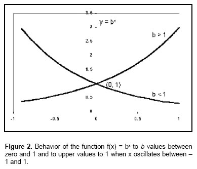
In general, in the functions of the form f(x) = xn J*, the n exponent is constant and the x base is variable. By changing the order of this function the base is the b constant and the exponent is the x variable, the following exponential function can be obtained: y = f(x) = bx K* in that b > 0 but b ≠ 1.
To b > 1, the function f(x) increases when x increases while 0 < b < 1, the function f(x) diminishes when x increases (see Figure 2).
In all cases, this exponential function shows the following characteristics: 1) it does not exist intersection with x because it does not exist a value of x in that bx is zero, 2) the intersection in y is (0, 1), 3) PC degradability, PC % the y values are in the positive quadrants, 4) the x axis is asymptotic, 5) while the dominium elements of f(x) = bx change arithmetically, the elements associated to the range, change geometrically. So, the geometric progression of values of f produces a tendency to increase (or to diminish) which is very important when the base is the e constant (10).
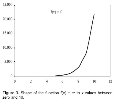
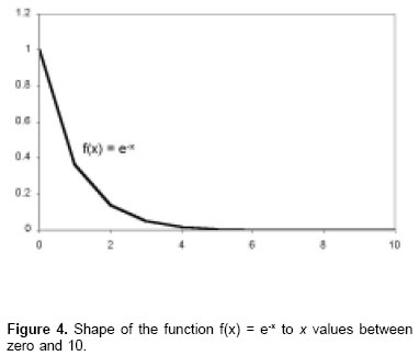
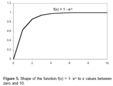
Due to its fundamental importance in several biologic phenomena, the f(x) = ex function is called “natural exponential function” (23). In Figure 3 it is observed that when x increases, the function increases also. However, this function can be inverted becoming negative the x exponent, so: f(x) = e-x L*.
In this equation, when x increases, the function decreases with values that oscillate between 1 to x = 0 and the limit value is zero when x tends to infinite (see Figure 4). Subtracting 1 of this equation it is obtained a graphic as is observed in Figure 5 and whose values are inverted in comparison to L* equation, this is, the values oscillate between zero to x = 0 and the limit value of 1 when x tends to infinite. Substituting the independent LL* x variable as the time t, it is obtained, f(t) = 1 - e-t LL*.
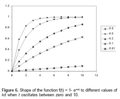
Incorporating a constant (kd) associated to t exponent, the equation LL* is modified:
f(t) = 1 - e-kdt M*.This constant had received different names and had been denominated in several ways. Thus, Ørskov and McDonald (19), and Jessop (9) denominated it as constant fractional rate of degradation, Mertens (13) denominated it as fractional rate of digestion, whereas Sniffen et al (21) called it specific rate of ruminal digestion, Bach et al (3) constant rate of degradation, Gómez and Van Der Meer (6) degradation velocity, and Galyean and Owens (5) denominated it as constant rate of digestion.
To Mertens (13), kd is the proportion of mass in a pool that changes per unit time while to Jessop (9) is a measure of the proportional change in some constituent. In the other hand, Galyean and Owens (5) interpreted it as the ruminal degradation velocity indicating that when kd takes a value of 0.04%/h, 4% of the constituent is digested each hour.
This denominations are not accurate and, besides, misunderstood.
If 0 < kd < 1, as while kd tends to zero, the response in the equation M* is reduced proportionally with the kd value (see Figure 6). Thus, kd determines the diminishing rate in the increase in the response of the equation M* while the independent variable t increases and it is equivalent to the instantaneous declinig rate of marginal productivity in the Thünen’s model.
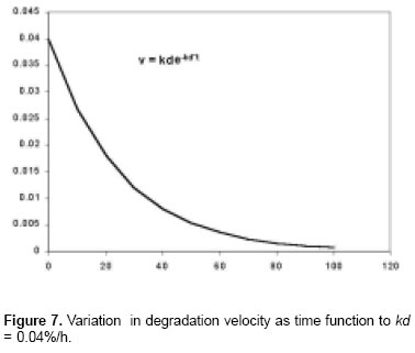
To understand the meaning of the kd constant, is necesary to carry out the next analysis: the first derivate on the equation when kd values, is f’(t) = kde-kdt = v(t) N*.
By definition, the first derivate of any function is equal to the velocity and its units are %/h. As it is appreciated in equation N*, the velocity of equation M* is variable showing a decrease exponential behavior (see Figure 7).
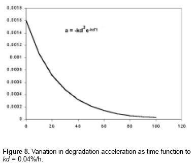
The second derivate of any function is, by definition, the acceleration and its units are %/h2. So, the second derivate of the equation M*, is f’’(t) = -kd2e-kdt = a(t) O*.
In Figure 8 it is appreciated that as the velocity, the acceleration is also variable and shows a decrease exponential behavior.
Dividing the acceleration on velocity, it is obtained -kd2e-kdt/kde-kdt = -kd P*.
This means that kd is the relationship between the ruminal degradation acceleration and its velocity and IT is expressed as 1/h.
This is also possible to demonstrate by obtaining the derivate of the natural logarithm of the absolute values of both members of the equality in the equation N*:
ln|v| = ln|-kd| + ln|e-kdt| Q*
ln|v| = -kdt R*
The derivate of this equation respect to t, is v’/v = -kd = a/v RR*.
Due that kd represents the constant quottient between two parameters of ruminal degradability kinetic (acceleration and velocity), a correct denomination to kd is constant kinetic of ruminal degradability.
Due to one of the characteristics of equation M* is to increase the value of the function to the limit of 1 while the independent variable t increased, when this equation is multiplied by a constant (B), the value taken by this constant will be the maximum value possible that can reaches the equation M*. So, this equation S* assumes the form RDb(t) = B*(1 - e-kd*t) .
The equation M* is similar to equation G*, therefore, it posses the same properties, this is, the product is zero when either factor is zero and the product is near the maximum value B when all factors increase to infinity. This constant corresponds to potentially degradable fraction in ruminal kinetic studies and the equation S* estimates the rumen degradability of B fraction (RDb).
The inclusion of an independent term (A) in the equation S*, allows to estimate the value assumed by this function when the independent variable (time) is zero and corresponds to the soluble fraction which is immediately degraded in the rumen:
RDA+B(t) = A + B(1 - e-kdt) T*.
Natural exponential equations have, in essence, the same properties of equation S*. This is the case of Grovum and Williams (7) model’s for the study of ruminal passage kinetic and, therefore, the constant of ruminal passage (kp) estimated by this model also represents the quotient between the acceleration and velocity of ruminal passage.
From the equation T* it is possible to estimate three parameters: the initial velocity, the initial acceleration and the time-life. The initial velocity (vo) is obtained as the first derivate of equation T* and resolving t = 0: vo = kdB U*.
In the same manner, the initial acceleration (ao) is obtained from the second derivate of this equation and resolving t = 0: ao= kd2B V*.
The time-life is the time necesary for a proportion (P: in percent/100) of initial quantity of the B fraction disapearing by degradation. To estimate this parameter is necesary calculate the t in that RDb is B*P, this is:
RDb(t) = B(1 - e-kdt)= B*P = 1 - P = e-kd*t W*.Appling the natural logarithm to both members of the equality (23), it is obtained -kdt = ln(1-P) X*. Then, reorganizing this equation the result is t = -ln(1-P)/kd.Y* Thus, to meet the half-life of B fraction (B*0.5), the equation is: t = -ln(0.5)/kd Z*.
Discussion
An adequate interpretation of mathematical model components is fundamental to its correc t application in estimation procedures. Since Ørskov and McDonald (19) applied the Thünen´s exponential model to estimate the ruminal degradability parameters, it had been an unclear interpretation of kd component of this model, which had received different names and had been denominated in several ways. It is incorrect to assume that this constant corresponds to velocity (rate). As it was demonstrated here, kd is the quotient between the rumen degradability acceleration and velocity which is different to the equation utilized by López et al (11) to calculate the kd in the simple negative exponetial curve model such of Thünen´s model. These autors utilized the negative quotient between the first derivate of equation OJO on the original equation assuming that kd is a function of the incubation time. This is incorrect, since as was demostrated here, kd is a constant that is unvariable over time. Its components, the acceleration and the velocity, are variable over time but keep a constant relationship.
The utilization of kd to estimate other parameters assuming that kd is velocity, therefore, it had led to mistakes. Such is the case of effective degradability (26) and dry matter intake (4). In this sense, it is necesary to review the calculus to estimate these other parameters and propose other methodologies coherent with kinematical characteristics of rumen degradability and passage.
Some authors assume that kd units are %/h (3, 8, 13). However, as was demostrated here, its unit is 1/ h. This is the same unit utilized by López et al (11) to kp in an equivalent equation utilized to estimate kd.
The initial velocity and the initial acceleration are parameters that allow to analyze in detail the kinetic characteristics of ruminal degradation of nutrient and do better formulation eschemes based on the synchrony of this parameters to diferent nutrional fractions such as crude protein and nonfiber charbohydrate (16).
In the other hand, the time-life is an important parameter: in other knowlodge areas, such as radioactivity. The half-life is a parameter applied to estimates the necessary time so that a sample of a radioactive isotop can be reduced at half (23). Although this parameter had been applied to ruminal degradability of nutrient, its value is less important than in radioactivity due that in the first case the nutrients are submited to other force besides of the degradation (the passage), so in some situations it is possible that B fraction dissapears totally before reaching the half quantity, while in the second case, the radioactive isotop is only affected by its radioactivity and its half quantity is always reached.
Conclusion
The model described by Ørskov and McDonald (19) to analyze data from in situ rumen degradability technique was originally proposed by Johann Heinrich von Thünen to study the responses of harvests to different production factors called the constant k as the instantaneous rate of decreasing in the marginal productivity. In the study of ruminal degradability kinetics of nutritional fractions, this constant is denominate kd, that along with the ruminal passage constant (kp), had been erroneously defined and estimation of other parameters such effective misunderstood as velocity parameter (rate). However, degradability (26) and dry matter intake (4) based in as it was demonstrated here, this constant represents this constant are mistaken and need to be reviewed to the quotient between the acceleration and velocity of propose other coherent methodologies with its degradation and passage, respectively. Therefore, the kinematical characteristics.
Acknowledgment
Specials thanks to Fernando Puerta and Jorge Cossio (Mathematics Department, National University of Colombia, Medellín Campus) for their mathematical assistance.
Resumen
Origen y estudio comprensivo del modelo Thünen para analizar datos de la técnica de degradabilidad ruminal in situ.
El modelo clásico utilizado para analizar datos de la técnica de degradabilidad ruminal in situ fue propuesto originalmente por Thünen para el estudio de la respuesta de los cultivos a diferentes factores de producción. Con la finalidad de establecer el significado de la kd en el modelo de Thünen, se realizó un análisis matemático que indicó que esta constante representa el cociente entre la velocidad y la aceleración de la degradación ruminal. De manera similar, la constante kp representa el cociente entre la velocidad y la aceleración del pasaje ruminal.
Palabras clave: aceleración, derivación, modelos exponenciales, velocidad
References
1. Agricultural and food research council. Nutritive requirements of ruminants animals: protein. Nutrition Abstracts and Rev. (Series B) 1992; 787 - 835. [ Links ]
2. Alexandrov AN. Effect of ruminal exposure and subsequent microbial contamination on dry matter and protein degradability of various feedstuffs. Anim Feed Sci Tech 1998; 71: 99 - 107. [ Links ]
3. Bach A, Stern MD, Merchen NR, Drackley JK. Evaluation of selected mathematical approaches to the kinetics of protein degradation in situ. J Anim Sci 1998; 76:2885-2893. [ Links ]
4. Ellis WC. Determinants of grazed forage intake and digestibility. J Dairy Sci 1978; 61: 1828 - 1840. [ Links ]
5. Galyean ML, Owens FN. Fermentation, digestion and passage in ruminants fed roughage and concentrate diets. In: Proc Of the Southwest nutrition and management conference. Univ of Arizona, Tucson; 1988. p 78 - 97 [ Links ]
6. Gómez A, Van der Meer JM. Velocidad de degradación de la materia orgánica y de la fracción NDF de la paja de cebada: efecto de la variedad y del tratamiento con amoniaco sobre la degradación "in vitro" e "in saco". Inv Agr: Prod Sanid Anim 1988; 3: 195 - 205 [ Links ]
7. Grovum W L, Williams VJ. Rate of passage of digesta in sheep. 4. Passage of marker through the alimentary tract and the biological relevance of rate constants derived from changes in concentration of marker in faeces. Brit J Nutr 1973; 30:313- 329 [ Links ]
8. Humphrey TM. Algebraic production functions and their uses before Cobb-Douglas. Economic Quarterly 1997; 83: 51 - 83. [ Links ]
9. Jessop N. Comparative Nutrition 3M. Course on line 2002; URL: http://helios.bto.ed.ac.uk/bto/biology/compneut/CourseInfo/courseinfo.html [ Links ]
10. Kovacic ML. Matemática; aplicaciones a las ciencias económico-administrativas. Fondo Educativo Interamericano, Colombia; 1977. [ Links ]
11. López S, France J, Dhanoa MS, Mould F, Dijkstra J. Comparison of mathematical models to describe disappearance curves obtained using the polyester bag technique for incubating feeds in the rumen. J Anim Sci 1999; 77:1875- 1888. [ Links ]
12. Marín MP, Cabrera R, López A, Bas F. Estudio comparativo de la degradabilidad in situ de la materia orgánica de cuatro forrajes en alpacas y cabras. Cienc Inv Agr 1997; 24: 25 - 34. [ Links ]
13. Mertens DR. Rate and extend os digestión. In: Forbes JM, FranceJ (eds), Quantitative aspects of ruminant digestion and metabolism. CAB International; 1993. p. 13 - 51. [ Links ]
14. Mitscherlich EA. Des Gesetz des Minimums und das Gesetz des abnehmended Bodenertrages. Landwirsch Jahrb 1909; 3: 537-552. Citado por: Humphrey TM. Algebraic production functions and their uses before Cobb-Douglas. Economic Quarterly 1997; 83: 51 - 83. [ Links ]
15. National research council. Nutrient requirements of dairy cattle, 6th rev ed Washington, D.C; National Academy Press; 1989. [ Links ]
16. National research council. Nutrient requirements of dairy cattle, 7th rev ed Washington, D.C; National Academy Press; 2001 [ Links ]
17. Nocek JE. In situ and other methods to estimate ruminal protein and energy digestibility: A review. J Dairy Sci 1988; 71: 2051-2069. [ Links ]
18. Ortega ME, Mendoza G, Aguirre S, Carranco ME. Tratamiento con formaldehído de maíz y sorgo, efecto sobre la degradabilidad ruminal de la materia seca, almidón y proteína bruta. Inv Agr: Prod Sanid Anim 1998; 13: 13 - 19. [ Links ]
19. Ørskov ER, McDonald I. The estimation of protein degradability in the rumen from incubation measurements weighted according to rate of passage. J Agric Sci 1979; 92:499- 503. [ Links ]
20. SAS/STAT User's Guide: Statistics, Version 6, 4th edition. 1989. SAS Inst., Inc., Cary, NC. [ Links ]
21. Sniffen CJ, O'Connor JD, Van Soest PJ, Fox DG, Russell JB. A net carbohydrate and protein system for evaluating cattle diets: II. carbohydrate and protein availability. J Anim Sci 1992; 70:3562-3577. [ Links ]
22. Spillman WJ. The law of diminishing returns. Yonkers-on- Hudson, NY: World Book Co, 1924. Citado por: Humphrey TM. Algebraic production functions and their uses before Cobb-Douglas. Economic Quarterly 1997; 83: 51 - 83. [ Links ]
23. Thomas GB. Cálculo infinitesimal y geometría analítica. Ed Aguilar, Madrid; 1959. [ Links ]
24. Thünen, JH von. Der isolierte staat in beziehung auf landwirthschaft und national okonomie. 3 volumes. Jena, Germany: Fischer, 1930. Citado por: Humphrey TM. Algebraic production functions and their uses before Cobb- Douglas. Economic Quarterly 1997; 83: 51 - 83. [ Links ]
25. Waldo, DR. Factors influencing voluntary intake of forages. In: Barnes RF et al (editors). Proceedings of the national conference on forage quality and utilization. Lincoln, Nebraska; Nebraska Center for Continuing education, Lincoln; 1970. p. E1-22. [ Links ]
26. Waldo DR, Smith LW, Cox LE. Model of cellulose disappearance from the rumen. J Dairy Sci 1972; 55: 125 - 129. [ Links ]

