


 English (pdf)
 Article in xml format
 Article references
 Send this article by e-mail
 Cited by SciELO
  Cited by Google
  Similars in
SciELO
Similars in
SciELO  Similars in Google
 Permalink
Introduction
For numerous applications, including chemical processes, it is well known that nonlinear state observers, parameter and unknown inputs estimators have been becoming of great interest. The main uses for those methods are the design of observer-based controllers, the synthesis of fault detection and isolation methods 1, among other applications. An important class of nonlinear observers is the Sliding Mode Observers (SMO) 2,3,4, which have the main features of the Sliding Mode (SM) algorithms. Those algorithms, are proposed with the idea to drive the dynamics of a system to a sliding manifold, that is an integral manifold with finite reaching time 5, exhibiting very interesting features such as work with reduced observation error dynamics, the possibility of obtain a step by step design, robustness and insensitivity under parameter variations and external disturbances, and finite-time stability 2,6. In addition, the last feature can be extended to uniform finite time stability 7 also known as fixed-time stability 8, allowing the controllers and estimators to converge with a settling-time independent to the initial conditions. On the other hand, it is said usually that the sliding mode algorithms present two main disadvantages:
they are usually assumed to be more sensitive to noise than linear controllers and estimators 9, and
the so-called chattering which is a high frequency oscillation due to the effect of discontinuities of the functions used to induce sliding modes (e.g. the sign function) on the unmodeled dynamics of the system 2.
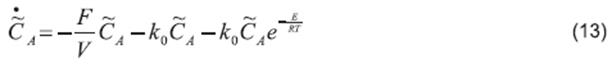
However, for the disadvantage (i), using the steady state error as performance index, it is shown that,under the bounded disturbance hypothesis, linear and discontinuous algorithms are equally sensitive to noise. Therefore, discontinuous algorithms are a better choice under both noise and disturbance presence conditions 10. Besides, for the disadvantage (ii), several approaches have been proposed to reduce or avoid chattering. A first example is the use of continuous and smooth approximations of the sign function as linear saturation or sigmoid functions 11, with this solution only a quasi-sliding motion can be forced in a vicinity of the desired manifold, decreasing the performance and the robustness of the algorithm 12. Another approach to induce sliding modes reducing chattering is to use continuous but nondifferentiable functions or with discontinuous derivatives, instead of a discontinuous function. These methods are the so-called High Order Sliding Mode (HOSM) algorithms 13, extending the idea of the SM actuating on the time derivatives of the sliding manifold, preserving the main features of the original SM approach. In addition, for a SMO design case, the chattering reduces to a numerical problem 14. Hence, some SMO have attractive properties similar to those of the Kalman filter but with simpler implementation 15. For chemical processes, SM observers have been applied for several cases. Some examples are shown in 16,17,18,19. The idea of coupling an observer with an Observer-Based Estimator (OBE) was used in 21 and, the idea of applying a High Order Sliding Mode Observer (HOSMO) for state and parameter estimation in a Continuous Stirred- Tank Reactor (CSTR), assuming the parameter to be estimated as an unknown input, was introduced by 21. Here, measuring the temperature inside the reactor, the observer estimates the heat of reaction, and the concentration of the reactive. In addition, in order to facilitate the estimation procedure, the global heat transfer coefficient was assumed to be a known constant. No dynamics of the temperature inside the jacket were considered in the mentioned approach. This paper proposes an extension of the last approaches, considering the global heat transfer coefficient as an unknown parameter to be estimated. This assumption conduces to a better approximation of the CSTRreal operation conditions. As a first step, an OBEfor the global heat transfer coefficient estimation isused. With this estimation, a HOSMO for state andinput estimation 22 is used to estimate the heatof reaction, and the concentration of reactive. Theheat of reaction is a parameter which is consideredto be an unknown input for the observer design.The HOSMO is based on a real-time differentiator23. In the following, the next section presentsthe mathematical model of the CSTR. Then, theestimation structure will be described. The paper continues with the results of numerical simulation.Finally, the conclusions of this paper are presented.Mathematical Model for the CSTR The CSTR considered performs an exothermic chemical reaction from the reactant Г to the product Ф(Г→Ф). This plant has also a recirculation flow in the jacket, which allows improving its controller design 24. The state equations of the CSTR are presented in two subsystems as follows, with the outputs T and Tj:
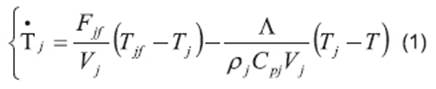
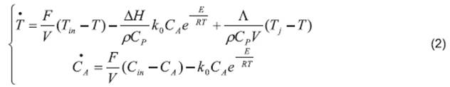
Here, F is the flow into the reactor, V is the volume of the reaction mass, Cin is the reactive input concentration, CA is the concentration of the reactive inside the reactor, k0 is the Arrhenius kinetic constant, E is the activation energy, R is the universal gas constant, T is the temperature inside the reactor, Tin is the inlet temperature of the reactant, ∆H is the heat of reaction (being an exothermic reaction, this corresponds to the released energy during the reaction), and in this article is considered an unknown input because it is an uncertain parameter, ρ is the density of the mixture in the reactor, Cp is the heat capacity of food, the parameter Λ=UA is the global coefficient of heat transfer, where U is the overall coefficient of heat transfer and A is the heat transfer area, Tj is the temperature inside the jacket, Fjf is the feeding flow, Vj is the jacket volume, Tjf is the inlet temperature to the jacket, ρj is the density of jacket flow, and Cpj is the heat capacity of the jacket flow (24).
Estimation System Design
In this section the estimation system for the CSTR is proposed, it estimates the following variables:
The concentration of the reactant inside the reactor, CA (state variable), due to expensive sensors.
The global coefficient of heat transfer, Λ (parameter), which depends on tank level (although in this paper it was considered constant), the stirring speed inside the reactor, the cleaning degree of the surface inside the reactor, and speed of the cooling flow inside the jacket; making its estimation a hard task 25.
The heat of reaction, ∆H (parameter), which is uncertain due to experimental measurement complexity of thermal and kinetic phenomena that involve it 18.
Considering Subsystem (1), it can be noted that the global coefficient of heat transfer, Λ, is the only unknown parameter.
Taking advantage of this characteristic, an estimation system based on cascade connection of an OBE with a HOSMO is proposed as follows:
Using measurements of T, Tj and, an OBE based on Subsystem (1), an estimation of the parameter Ʌ , , is obtained.
Using measurements of T,
Tj
, the estimated parameter and, a HOSMO based on Subsystem (2), estimations of the state variable
CA
 , and the parameter ∆H
  are obtained.
For the last case, the HOSMO structure allows to consider the parameter ∆H as an unknown input.
With this assumption, the estimation system is robust against variations of ΔH.
The whole structure for state and parameter estimation of CSTR is shown in Figure 1.
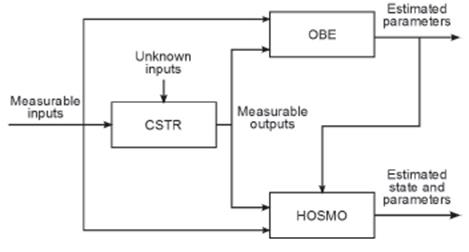
Regarding the cascade structure of the estimation system, it will be started with the parameter Λ estimation.
At first, it must be noted that the HOSMO allows the joint estimation of state and parameters, considering the last ones as unknown inputs.
However, it is no possible to fulfill the requirement by the HOSM in order to estimate simultaneously the parameters Λ and ΔH.
Therefore, the use of an OBE to estimate Λ is proposed here. Initially, it is highlighted that the proposed scheme, in addition to the temperatura measurement T, also requires an estimation of its time derivative . Ṫ
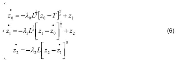
This estimation is performed by using a robust xact sliding mode differentiator 23, with the following structure:
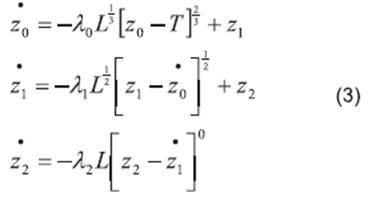
where it is defined the function ⌊•⌉α =|•|α sign (•)for α ≥ 0; z0 is the estimation of T, z1 is the estimation of its time derivative and, z2 is the estimation of , with λ0, λ1, λ2 being positive gains. Let the third derivative T(3) be bounded as | T(3) |< δT for all the time with δT a positive constant, therefore, the gain
L must be such that L> δT.
Note that a second order differentiator is used instead of a first order one, the variable z2 is not used, the main reason for this selection is to reduce the presence of numerical chattering on the estimated variables.
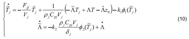
OBE design
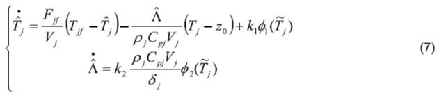
Taking into account the Subsystem (1) and using the jacket temperature equation Tj as coupling equation to calculate Λ, an OBE based on the generalized super-twisting algorithm 7 is proposed as follows:
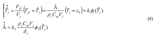
where .
 The OBE input injections are given by
 and,
and,
 with μ≥0. Finally, k1 and k2 are the OBE gains. The gain δj is a positive constant which takes the value of a lower bound for |z0-Tj|, the existence of this parameter is verified taking into account that all the temperatures are measured in Kelvin degrees and he condition z0>Tj for all the time.
Note that the system (4) can be considered as a second order sliding mode extension of the linear OBE presented in 26.
HOSMO design
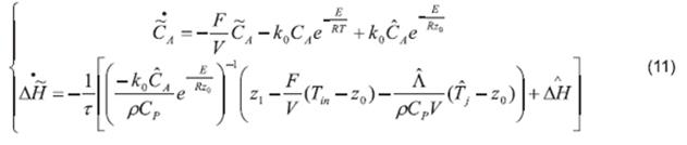
Once the estimation of Λ is obtained, a HOSMO of the form presented in 22 is designed based on Subsystem (2). This observer provides an estimation of the state variable
CA
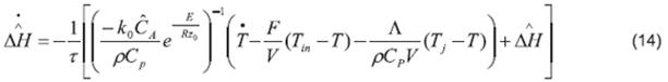
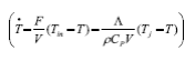
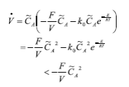
and the parameter ∆H. For this case, the parameter ∆H is considered as an unknown input. It is observed that the output T has a relative degree equal to one with respect with the unknown input ∆H, therefore ∆H can be written in terms of T and its time derivative  as follows from (2).
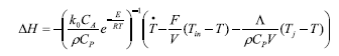
wThus, calculating the time derivatives of the output T using the robust exact sliding mode differentiator (3) , the HOSMO structure is
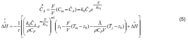
Where  is the estimation of ΔH.
Complete estimation scheme
From (4)-(3), the complete estimation scheme is given by the following system:
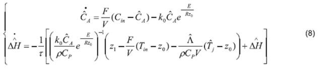
which is a coupled system formed of seven differential equations.
Convergence analysis
The convergence analysis for the system (6)-(8) is performed by analyzing the stability of the error system.

Where
 and .
and .

At first, for the system (9), with the third derivative T3 be bounded as | T3 |< δT for all the time and L > δT , the errors  converge to zero in a finite time tj > 0 24.
Now, for the system (10), let =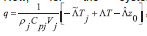 , hence
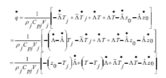
Therefore, from (4) and (10), it follows:
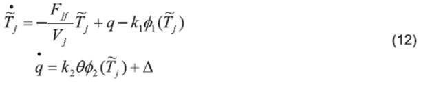
Where
 and
and
 is an
is an
unknown but bounded perturbation,  for all the time, with a positive constant.
If the gains k1, k2 are in the set the system (12) is fixed-time stable 7, that is a sliding mode appearson the manifold ( ,q)=(0,0) in a fixed time tq>0.
In this form, with tjq= max (tj , tq), a sliding mode appears on the manifold  in a finite time tjq >0.
The motion on the sliding manifold  = (0,0,0,0,0) is given by
Taking into account that (14) is just a first order low-pass filter for the estimation of ΔH given by
the stability analysis is completed considering the equation (13). Thus, let the Lyapunov function
Therefore, the error  is exponentially stable to the equilibrium point zero.
Numerical Simulation Results
The numerical simulations results of the proposed estimation structure applied to a CSTR are presented in this section. All simulationspresented here were conducted using the Euler integration method, with a fundamental step size of 1 × 10⁻⁴ [min]. The CSTR parameters are shown on Table 1.
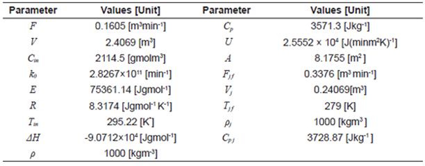
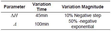
In order to verify the observer performance in presence of parametric variations, the changes shown in Table 2 were introduced in the simulation. Is worth to notice that this changes are unknown for the proposed estimation system.
The initial conditions for the CSTR were selected to:Tj(0)=284.084[K], T(0)=314.7208[K] and;
CA
(0)=907.1774[gmolm3] and for the observer to: (0)=286.9248[K],  (0)=1.8801×10⁵[J.(minK)-1], (0)=997.8951[gmolm-3],
z0
(0)=314.7208[K], z1(0)=0[Kmin-1], z2(0)=0[Kmin2] and (0)=-9×10⁴[Jgmol-1]. For the OBE the selected parameter values were adjusted to:
k1
=3.4026,
k2
=5.9821×10⁴ and µ=1. For HOSMO, the parameters
λ0
=2,
λ1
=1.5,
λ2
=1.1 and L=10 were used. Finally, the filter constant was adjusted to:
(0)=1.8801×10⁵[J.(minK)-1], (0)=997.8951[gmolm-3],
z0
(0)=314.7208[K], z1(0)=0[Kmin-1], z2(0)=0[Kmin2] and (0)=-9×10⁴[Jgmol-1]. For the OBE the selected parameter values were adjusted to:
k1
=3.4026,
k2
=5.9821×10⁴ and µ=1. For HOSMO, the parameters
λ0
=2,
λ1
=1.5,
λ2
=1.1 and L=10 were used. Finally, the filter constant was adjusted to:  .
.
This section is divided into two parts. In the first part, there is assumed that the temperature measurements are noiseless; in the second part instead, there is included a normally distributed random signal as measurement noise in the temperature.
Noiseless measurements
In this subsection, there is assumed no noise in the measurements.
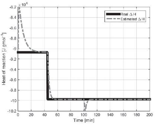
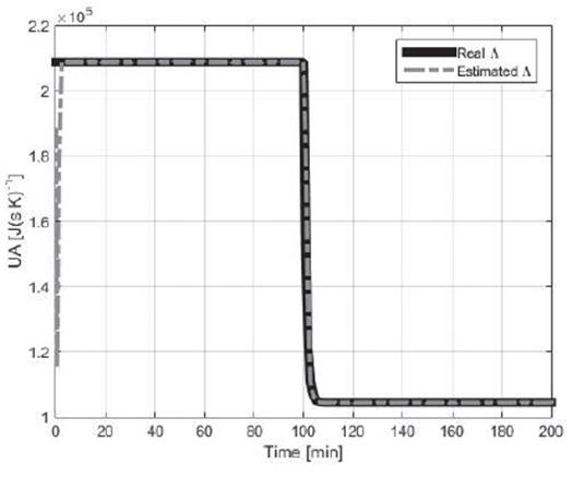
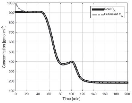
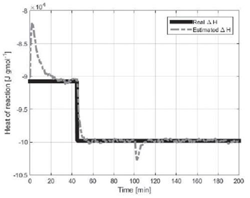
Figures 2 to 4 show the concentration of reactive inside the reactor
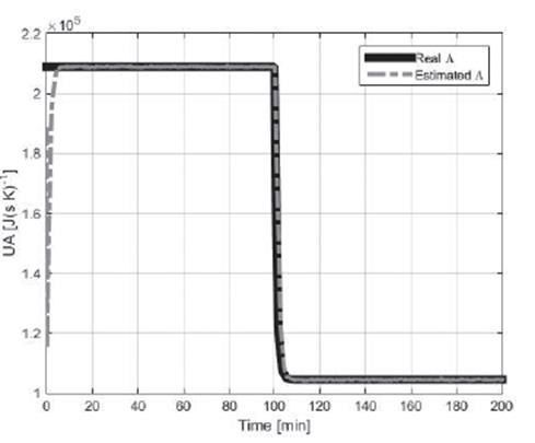
CA
, the heat of reaction  and the global coefficient of heat transfer Λ, respectively, for noiseless measurements.
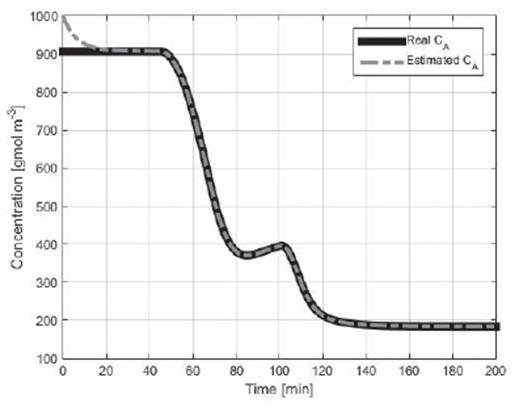
The estimated concentration converges to the actual concentration, with a settling time of approximately 20min (see Figure 2). Then for changes in both parameters it can be noted that the estimate of the concentration remains correct (t=45min y t=100min), which shows that the scheme of Figure 1 is robust with the parametric scheme of Figure 1 is robust with the parametric changes. That is, for parametric changes the observer responds correctly, estimating the variable of interest without steady-state error.
Likewise, Figures 3 and 4 show the correct estimation of the parameters for changes in the initial condition and changes in the process.
Noisy measurements
In this subsection, there is assumed that the temperature measurements were corrupted by a normally distributed random signal with zero mean and 0.1111 variance; this assumed variance responds to the fact that many temperature sensors report an accuracy of ±1[K].
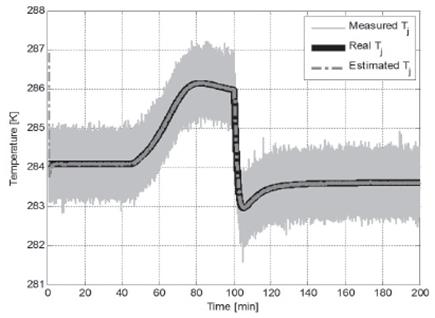
Figures 5 to 8 show the temperature inside the jacket
Tj
the concentration of reactive inside the reactor
CA
, the heat of reaction  and the global coefficient of heat transfer Λ, respectively, for noisy measurements.
Based on the presented figures, a good performance of the proposed scheme is observed, also under noisy measurement conditions.
The measurement noise is filtered by the estimation algorithms (Figure 5), this way the estimated concentration convergence is similar to the noiseless convergence.
Also the fast and accurate convergence of the estimated parameters can be highlighted, although a little deviation is noted in the estimated heat of the reaction due to the high gain of the observer for this case. The HOSMO presents a correct estimation due to its capacity to calculate the parameters (Figures 7 and 8).
In addition, the simultaneous estimation of ∆H and Λ using the OBE makes the proposed system robust against this parameter variations under noise conditions, the estimated temperature inside the jacket is much closer to its real value than its measurement (Figure 5) and the estimated concentration remains correct, without steady-state error. Similarly to the noiseless measurements case the scheme is robust with the parametric changes.
Besides, it can be noted that the HOSMO presents reduced chattering due to the use of the second order differentiator; with this proposal, all discontinuities that produce chattering come up at the second time derivative, not at the first which is used in the estimation.
Conclusions
An estimation structure for a CSTR based on a second order sliding mode extension of an OBE coupled to a HOSMO was proposed. This scheme, apart from allowing state estimation, allows estimating two parameters of the process, which are well known as very difficult to measure, especially for real-time applications. One of these parameters was considered as an unknown parameter in the HOSMO, and the second one is estimated by a second order sliding mode OBE. Hence, this configuration ensures a state estimation that is robust against variations of the mentioned parameters. With a suitable selection of the observer parameters, the structure presents a fast convergence with high accuracy.
Numerical simulations show a good performance of the proposed approach, exposing some features as the accurate estimation of both parameter and state, robustness against these parameter variations, and a short-time convergence of the whole system, also under noisy-measurement conditions. Furthermore, the proposed estimation scheme presents reduced chattering presence due to the use of a second order differentiator instead of a first order one. The proposed approach can be extended to more complex processes with similar structures. For these cases, the computational burden can increase.

