Estimating Volatility Returns Using ARCH Models. An Empirical Case: The Spanish Energy Market

Una estimación de la volatidad de los retornos empleando modelos ARCH: El caso del mercado energético español

Une estimation de la volatilité des rendements en utilisant un modèle ARCH : Le cas empirique du marché espagnol de l’énergie

Ricardo Alberola

Ricardo Alberola Gallardo: MSc. in Economics Science and Teaching Assistant at FAE, University of Alicante (Spain). Currently, the author is Financial Analyst at Caja de Ahorros del Mediterráneo (CAM). E-mail: ralberola@cam.es. Contact address: C/avda, Constitución 21, 3o 03660 Novelda. Alicante, España. I am especially grateful to Mª ángeles Carnero who has been my tutor. I am very grateful to my friends Jorge Barrientos-Marin, Alicia Perez and Szabolcs Sebestyén. An especial deserves the department of FundamentosdelAnálisisFundamentos del Anáálisis Económicoo(FAE) foritsfinancialsupport.ToarrivetothismomenthasbeenhardandI (for its financial support. To arrive to this moment has been hard and I would like to remember my parents.

-Introduction. -I. Models. -II. Empirical Results. -Conclusions. -References. -Appendix.

Primera versión recibida en abril de 2006; versión final aceptada en noviembre de 2006

Resumen: Este artículo analiza las regularidades más comunes en las series de tiempo del rendimiento diario de las acciones del mercado de energía de España, desde un punto de vista empírico. Al ser una herramienta poderosa para modelar su volatilidad, ajustamos una selección de procesos de heterocedasticidad condicional autorregresiva (ARCH) a las series. Se encuentra que solo dos series tienen una relación significativa, aunque diferente, entre el rendimiento condicional esperado de la acción y su varianza condicional: Enagas, cuya relación es negativa y Cepsa, cuya relación es positiva. Se encuentra, además, que el mercado eléctrico ha sido el más volátil durante el período analizado.
Palabras clave: series financieras, acciones, rendimiento, riesgo, volatilidad, modelos ARCH, puntos de cambio estructural. Clasificación JEL: C22.

Abstract: This paper analyzes the most common regularities of daily stock returns time series in the Spanish Energy Market from an empirical point of view. As they are a powerful tool, we fit a selection of developments of Autoregressive Conditional Heteroscedastic (ARCH) processes to the series in order to model their volatility. The paper finds that just two series have a significant and different relationship between the expected conditional stock return and its own conditional variance: Enagas (negative) and Cepsa (positive). It also finds that the electric market has been the most volatile market during the period under analysis.
Keywords: financial series, stock, return, risk, volatility, ARCH model, structural change points.

Résumé: Cet article analyse, du point de vue empirique, les fréquences les plus communes dans les séries de temps du rendement journalier des actions du marché espagnol de l'énergie. Etant donné qu il s'agit d'un outil puissant pour modeler leur volatilité, nous avons ajusté les séries à travers une sélection de processus d'heterocedasticité conditionnelle autorégressive (ARCH). Nous trouvons qu'il n y a que deux séries qu'on une relation significative mais différente entre le rendement conditionnel attendu de l'action et sa variance conditionnelle : il s'agit de Enagas dont sa relation est négative et Cepsa dont sa relation est positive. Nos trouvons également que le marché d'électricité a été parmi tous les plus volatil pendant la période d'étude.
Mots clés: séries financières, actions, rendement, risque, volatilité, modèles ARCH, points de changement structurel.

Introduction

In this work, we analyze empirically financial time series of returns in the Spanish Energy market. We model volatility by means of type ARCH processes in order to explain its regularities. Nowadays, risk and uncertainty play a central role in financial decisions. How asset returns are affected by arrivals of information and their non-trivial dependence on the past is a question with several answers in the literature. The search and selection of models able to reproduce asset returns regularities is still an objective.

Some of these regularities are well documented in the literature. For example, Mandelbrot (1963) and Fama (1965) observed that asset returns are not normal independently distributed. They have leptokurtic distributions meaning that large observations, in absolute value, occur more often than expected from a normal variable. This is also known as Thick Tails. Moreover, Mandelbrot (1963) documented that volatile periods, characterized by large returns in absolute value, tend to alternate with more quiet periods of smaller returns. This is the volatility clustering property of asset returns.

In 1982, Robert Engle introduced the Autorregresive Conditional Heteroscedasticity (ARCH) class of models to analyze time-varying volatility, where the conditional variance of returns at time t, σ_t², is a linear function of the past squared observations. Later, Bollerslev (1986) generalized the model of Engle by specifying the conditional variance as a linear function of squared laGed observations and laGed conditional variances, and independently, Taylor (1986) and Schwert (1989) modeled the conditional standard deviation as a linear function of past absolute observations and past standard deviations. Other parametrizations of volatility, which can capture these stylized facts of asset returns, are the non-linear (NARCH) model proposed by HiGins and Bera (1992), and the quadratic GARCH (QGARCH) model proposed by Sentana (1995).

Alternativelly, Taylor (1986) proposed the Autorregresive Stochastic Volatility model (ARSV) which specifies volatility at time t as a stochastic process. Although ARSV models are more flexible than ARCH; see Carnero et al. (2004a), their estimation is a much more difficult task contributing ARCH models to become a tool widely used for modeling volatility.

Since then and until now, a vast family of ARCH versions is the result of research focused on other empirical regularities of asset returns such as skewness. Two main theories have attempted to explain this skewness: On one hand, large negative returns seem to be more frequent than large positive ones. This fact produces negative skewness in market returns. Furthermore, volatility is usually higher after the stock market falls than after it raises. Therefore, volatility of returns has an asymmetric predictable response to the changes in stock prices: it increases more when stock prices fall than when stock prices raise, so that there is a negative correlation between volatility and returns. This is so-called leverage effect and was reported by Black (1976): when leverage of firms increases, uncertainty increases too. However, Black (1976), Christie (1982) and Schwert (1989) found empirically that leverage alone can not explain all the asymmetry. Asymmetric ARCH (AARCH) by Engle et al. (1990), Exponential GARCH model (EGARCH) of Nelson (1991), Threshold ARCH model (TARCH) proposed by Zakonian (1990) and its modified version of Glosten, Jagannathan and Runkle (1993) (GJR) are able to capture this predictable asymmetric effect.

On the other hand, many authors maintain the existence of a volatility feedback effect. French et al. (1987) used the Generalized ARCH in Mean (GARCH-M) model of Engle et al. (1987) in order to examine the intertemporal relation between risk and stock returns and conclude that there is a positive relation between the expected market risk premium and the predictable volatility of stock returns, unlike a negative relation between unexpected stock market returns and the unexpected change in volatility of stock returns. If volatility at a given moment is higher than predicted, then agents will revise upward future expected volatilities. If the risk premium is positively related to volatility, the discount rate of future cash flows will increase. If cash flows are unaffected, this higher discount rate reduces both their present value and the current stock price.

Campbell and Hentschel (1992) developed a QGARCH model for the news about future dividends of stocks and allowed them, its volatility and the revision from time t to t+1 of the discounted value of future expected returns to affect the actual expected stock returns. When large pieces of (positive or negative) news arrive, they tend to be followed by other large pieces of news, future expected volatility increases, given that agents are risk averse, bigger uncertainty requires higher expected stock returns and this lowers stock prices, amplifying the effect of bad news and dampening the good news one. In contrast, the arrival of a small piece of news lowers future expected volatility and increases the stock price.

Although the latter papers found a positive relation between expected returns and conditional variance using monthly data of the value-weighted portfolio of all New York Stock Exchange (NYSE) stocks and daily Standard and Poor s (S&P) composite portfolio data, from the Center for Research in Security Prices (CRSP), Nelson (1991) found a negative relation using daily returns for the value-weighted market index from the CRSP. In addition, Glosten et al. (1993) used a set of modified GARCH-M models and their results supported those of Nelson, with monthly data of the CRSP index. Unlike Chan et al. (1992), who used a bivariate GARCH-in-mean process and find no significant relation between expected returns and their own conditional variance for the U.S., they used daily S&P 500 stock index for U.S. and Nikkei and Morgan Stanley Japan and EAFE indices for foreign markets.

A more recent approach to explain skewness was developed theoretically by Hong and Stein (2003), and they supported this theory empirically with Chen et al. (2001). Their model explains how the degree of ex-ante investor heterogenity can lead to a positive unconditional skewness in the returns of an individual stock, this is frequent in empirical works, although returns of the whole market are usually negative skewed. Differences of opinion about the market are on average more pronounced than differences of opinion about individual stocks and negative asymmetries are more likely to occur.

It is an empirical fact that asset returns have little serial correlation but, far from being independent, transformations of them like 2tr or dtr (where 2tr is the return of a speculative asset), could have quite high autocorrelation for long lags decaying towards zero slowly. Ding et al. (1993) characterized this issue as a Long-memory property of asset returns being strongest for values of 1=dor near 1, and suGested an asymetric model called Asymetric Power ARCH (A-PARCH) in which the power of the conditional variance is a parameter. This avoids imposing some structure on the data squaring them or not as it is done in ARCH/GARCH and Taylor models. For a revision of other asset returns stylized facts like persistence of shocks to volatility or comovements, see Bollerslev et al. (1994) and Ghysels et al. (1996).

In the work presented here, we model volatility by means of ARCH models presented below, fitted to the stock market returns series in the Spanish Energy market. In section I we present the models used, in section II we describe the data analyzed and get empirical results. Finally, the last section concludes.

I. Models

In the GARCH (p,q) model, proposed by Bollerslev (1986), returns are assumed to be: r_t + ε_t with conditional mean v_t = E_t-1(r_t),and conditional variance σ_t² = Var_t-1(ε_t) changing over time. Innovations ε_t = σ_tz_t where z_t N(0,1) and independent of the second process σ_t known as volatility and satisfying

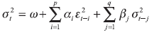(1)

in which all the coefficients must be positive, and the condition:

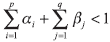
is needed for covariance stationarity.

From these assumptions and in order to capture more regularities like long memory and leverage effects in just one model, Ding et al. (1993) proposed the A-PARCH(p,q) model which includes several ARCH models as special cases. In this model, volatility s power is a parameter δ that can be estimated, i.e.

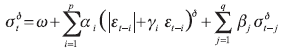(2)

With ω_i > 0, α_i ≥ 0, β_j ≥ 0, |γ_i| < 1, i=1,...,p, j=1,...,q. α_i and β_j are standard GARCH parameters and γ_i is the leverage effect parameter; it allows positive and negative innovations to have a different effect in the expected volatility. A conditional normal distribution is assumed for r_t, δ ≥ 2 and the expression

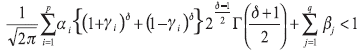
are sufficient conditions for covariance stationarity of ε_t. We shall refer to a version of the Eq. (2) in which the leverage effect parameters γ_i are zero for all i=1,...,p as a Power ARCH (PARCH) model.

Taylor (1986) and Schwert (1989) model conditional standard deviation as

(3)

Then, it is easy to see that, Eq. (2) encompasses Eq. (1) and Eq. (3) as special cases letting: γ_i = 0 for all i, and δ = 2 or δ = 1.

Different versions of the A-PARCH model lead to other ARCH models in the literature. In our study we also have used the above mentioned QGARCH (p,q) model proposed by Sentana (1995) which is not encompassed in the A-PARCH. In its general form, QGARCH is given by

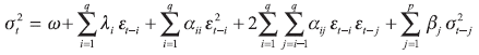
being covariance stationary if the condition ∑_i α_ij + ∑_j β_j < 1 holds. The cross product term, α_ij, gives the extra effect of interaction of laGed values of ε_t and λ_i parameters allow a dynamic asymmetric effect of positive and negative values of ε_t in σ_t². In this work we have used the simplest order one version QGARCH (1,1),

σ_t² = ω + λε_t-1 + αε_t-1² + βσ_t-1²

ARCH models with normal errors are often unable to capture all the leptokurtosis present in high frequency returns. To solve this problem, several authors proposed other distributions for z_t, for example a Student-t distribution with η > 2 degrees of freedom, see Bollerslev (1987), or the generalized error distribution (GED), see Nelson (1991).

A. Arch- in-Mean Models

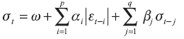
Many theories in finance involve an explicit tradeoff between the risk and the expected return. The ARCH-in-Mean (ARCH-M) model introduced by Engle et al. (1987) was developed to capture such relationship. In this work we use ARCH-M versions of the previous models in which the conditional mean is a linear function of the conditional variance of the process.

E_t-1(r_t) = v_t + Φσ_t²

Depending on the sign of Φ, an increase in the conditional variance will be associated with an increase or a decrease in the conditional mean. When dealing with market indices, Φ is seen as a measure of the risk aversion degree of agents.

II. Empirical results

In this section, we first describe the financial time series analyzed. Then, we get estimated daily volatilities for all series using different ARCH type models described in the previous section.

A. Series description

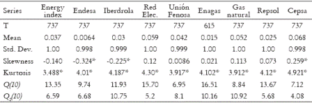
Our data have been sourced from the Madrid Market Data Base. They are daily stock prices for the index and enterprises of the Spanish energy market, more specifically the Energy Index, Endesa, Iberdrola, Red Eléctrica Española, Unión Fenosa, Gas Natural, Repsol and Cepsa, observed daily from January 3rd, 2002 to December 10th, 2004 for all series except for Enagas which has been observed from June 27th, 2002, to December 10th, 2004.¹

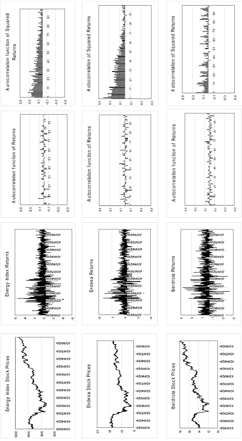
For each one, the series of daily financial returns have been calculated as r_t = 100*[log(s_t) - log(s_t-1)], where s_t is the closing stock price on day t. Appendix 1 contains plots of the series together with the correlogram of returns and squared returns. Table 1 contains descriptive statistics of the returns series. As we can see in this table, all returns series, with exception of Enagas and Cepsa, have a mean, which is not significantly different from zero. They are leptokurtic, with kurtosis coefficient bigger than 4, they present volatility clustering and most of them are serially uncorrelated. Also, most of the series present small significant serial correlation of squared returns decaying towards zero very slowly. All these features are empirical regularities of asset returns which are well documented in the literature, see for example Bollerslev et al. (1994) and Ghysels et al. (1996).

Table 1. Descriptive Statistics of the Returns Series

T: Sample Size. *Significant at 5%. Results for corrected series in parenthesis. rho;(10): returns autocorrelation of order 10. ρ₂(10): squared returns autocorrelation of order 10. Q₂(10) : Mcleod and Li statistic.

Looking at the plots, we can see that the Gas Natural and Cepsa returns series present one single large level outlier. This is important because, as it is the case, it may bias the sample statistics of the returns series. These outliers are the market response to unforecastable information. In the case of Gas Natural, in March 10th, 2003, Natural announces take-over bid for 100%% of Iberdrola (Diario Expansión, March 11th, 2003). Such announcement was not well received by the market. Repsol and BBVA² were not in agreement with it, and stock prices of Gas Natural fell, and the return fell dramatically too. In the case of Cepsa, in September 26th, 2003, BSCH³ announces take-over bid for 16%% of Cepsa (Diario Expansión, September 27th, 2003). This anouncement was well received and Cepsa s stock price increased. Because of this single outlier, the kurtosis coefficient of the contaminated series is severely distorted and the correlogram of squared returns is biased towards zero. Consequently, tests for conditional heteroscedasticity based on the autocorrelation function, like Mcleod and Li (1983) which uses Box-Ljung statistic for squared observations given by

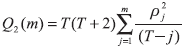
(T is the sample size) will be affected. Under the null hypothesis of conditional homoscedasticity, if the eight moment of r_t exists, Q₂(m) is approximately distributed as a χ₂² . Then Q₂(10) is approximately distributed as a χ₁₀² and the critical value under the null is 18.35. In both cases, Cepsa and Gas Natural, Q2 (10) is not significant at 5%% level and we can not reject the null. Furthermore, outliers are able to bias the parameters estimates and standard deviations of ARCH models; see Carnero et al. (2004b) where effects of outliers on the identification and estimation of conditional heteroscedasticity are analyzed. In order to avoid this issue, the series have been corrected by substituting outliers by the unconditional mean. Descriptive statistics of corrected Gas Natural and Cepsa series are given in parenthesis in Table 1, then the value of Q₂(10) turns to be significant and we reject the null hypothesis of conditional homoscedasticity in the series; see also the plot of corrected returns series and correlogram of corrected squared returns in Appendix 1.

By looking at the Repsol' s plot, we are able to appreciate that the returns series is much more volatile from the beginning of the period until the middle and then it becomes much quieter. A reason could be a significant change in the unconditional variance at a point of the series. It would be interesting to test this hypothesis and locate this point. We will turn to this question in Section II.B.2.

B. Estimation Results

In order to estimate daily volatilities of the stock returns series in the Energy market we fit models in section I to the returns series presented above. Although the Gaussianity assumption for the standardized innovations z_t is questionable,⁴ it is known that under suitable regularity conditions, Quasi-Maximum Likelihood estimators of the parameters are consistent and asymptotically normal; see for example Bollerslev and Wooldridge (1992) for the GARCH model. For every series our selection criteria was to choose the significant parameters and highest log-likelihood model, and from those models with the same log-likelihood, the simplest one was chosen. We report results for selected models in Table 2. Returns series do not present significant autocorrelation, then v_t was fixed and we found only significant value in the Enagas return series, v = 0.093, std.error = 0.0452 and t-statistic = 2.06.⁵ In order to ensure independency of standardized innovations, Box-Ljung and Mcleod-Li tests were applied to all the series, and the null hypothesis was not rejected for standardized residuals, see Table 3.

Table 2. Results for Selected Models

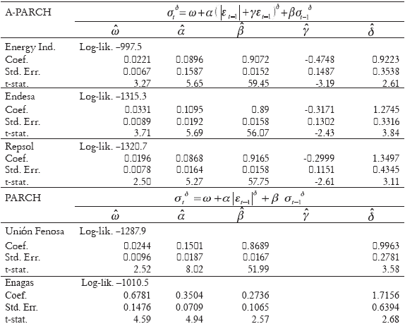
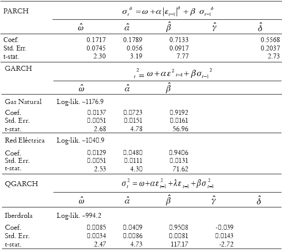
In the models with a significant power parameter we found δ smaller than 2, in concordance with Ding et al. (1993) results, and the asymmetric estimated parameter γ was significant, negative and in absolute value smaller than 1 for Energy Index, Endesa, REPSOL and Iberdrola. So negative returns increase expected volatility in contrast to positive ones which lower it. This supports a negative correlation between stock prices and predictable volatility of returns.

Figure 1 plots estimated volatilities of enterprises grouped by main business compared with estimated volatility of Energy Index. As we can see, in the first part of the period, the Electric market has been more volatile than Gas and Oil markets. It is clear there are 3 enterprises, Endesa and Union Fenosa in the Electric market, and Repsol in the Oil market, with the highest volatility. For all the other enterprises, estimated volatility has a similar behavior being around the Index one. In the second part of the period, estimated conditional standard deviations are similar for all enterprises and the Index, being lower than 2. The results for Repsol could be questionable if returns of Repsol present a change in the unconditional variance. In section II.B.2 we answer this question.

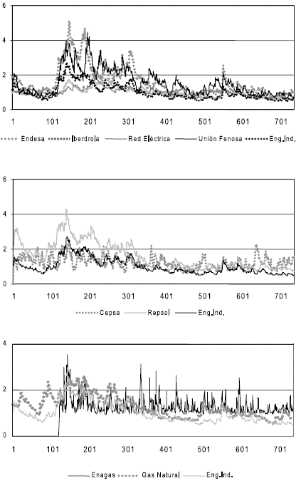
Figure 1. Standard Deviations

Table 3 contains descriptive statistics of standardized residuals. As it was expected, Mean and Standard Deviation are estimated close to 0 and 1, but, in the case of Endesa and Iberdola, residuals have negative skewness coefficient significantly different from zero still. This is a common feature of stock returns; large negative returns are more common than large positive ones. However, Cepsa has both standardized residuals and stock returns positive skewed. These results are in concordance with those of Chen et al. (2001). Then, the leverage parameter of Endesa ( γ ) and Iberdrola ( γ ) models can not capture all the skewness in the series, furthermore in the CEPSA case we do not find a significant leverage parameter. Campbell and Hentschel (1992) reported empirically that volatility feedback contribution to the variance of returns is small though it has an important effect on the skewness of returns.

Table 3. Standardized Residuals

Q(10): Box-Ljung statistic. *Significant at 5%

The reason for standardized returns have excess of kurtosis could be that returns would be not necessary conditionally Gaussian.

1. ARCH-M Results

We fit the ARCH-M version of the above models to our series looking for some relationship between returns and their own estimated conditional variance. We have found significance of the conditional variance parameter in the mean equation just for Enagas and Cepsa. Table 4 contains estimated parameters and Table 5 standardized residuals. A more accurate fit was reached with a QGARCH (1, 1)-M for Enagas returns series and a GARCH (1, 1)-M for Cepsa returns than with PARCH-M model (which was used in the previous section). Estimated conditional variances using these models in mean were very similar to the previous section ones.

Table 4. Estimated Parameters

Table 5. Standardized Residuals

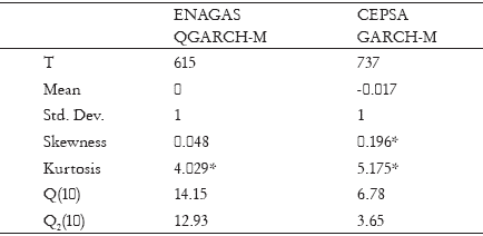
The Φ estimated parameter which measures the relationship between returns and conditional volatility has a positive sign in Cepsa unlike a negative sign in Enagas. This is not surprising because if agents are risk averse they require a larger expected return from an asset riskier within a period. However, across time this investors behavior is not clear. For instance, next two positions are equally acceptable. First, when agents are risk averse, they require a larger expected return when payoffs are riskier, leading to a positive sign of Φ. On the other hand, a larger expected return may not be required because investors may want to save more during riskier periods, leading to a negative sign of Φ, see Glosten et al. (1993). These authors argued that positive or zero relations between returns and volatility come from studies that use the standard GARCH-M model as French et al. (1987) did. In their work, et al. (1993), used standard M and got a positive correlation. However, they used Threshold GARCH model of Zakoian (1990) to allow positive and negative innovations to returns to have different impacts on volatility and they got a negative correlation. In contrast, Campbell and Hentschel (1992) using QGARCH (2, 1)-M, which captures predictable asymetries, found a positive correlation for daily excess stock returns. Our results are in agreement with Glosten et al. (1993) and against Campbell and Hentschel (1992).

For ENAGAS, v = 0.31, is 3.1 times bigger than its standard error unlike PARCH model where v =0.093 was 2 times bigger⁶ and standardized residuals are not significantly skewed, although kurtosis coefficient is smaller, leptokurtosis is still present. For CEPSA, the estimated GARCH-M model provides standardized residuals still positively skewed. The corresponding skewness coefficient is smaller in the M residuals than in the PARCH ones, unlike the bigger kurtosis coefficient. We have not been able to capture any predictable asymmetries of stock returns innovations to conditional variance with any asymmetric ARCH model. French et al. (1987) used GARCH-M with monthly data and found a positive correlation between the conditional mean and the conditional variance of stock market returns. They got negative skewness in the standardized residuals of GARCH estimation and argued it was due to volatility feedback effect. Given that the standardized residuals of PARCH and GARCH-M models are positive skewed, our results for CEPSA seem to be closer to those of Chen et al. (2001) where they empirically found positive skewness in individual stock returns, supporting Hong and Stein (2003) theory.

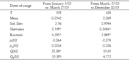
2. Repsol s Returns Serie

In Section II.A we proposed to test for a change in the unconditional variance of the Repsol s return series and locate the date when it happens. With this objective, we have applied the ICSS algorithm proposed by Incláán and Tiao (1994). With samples of random variables bigger than 200 observations and changepoints in the middle, as we suspect it is the case, this test reaches good results. It is more efficient in terms of CPU time than others like Likelihood Ratio tests and it is straightforward to compute.

The algorithm locates the change points of variance in a series of uncorrelated random variables,{r_t}, with mean 0 and variances σ_t², by maximizing the absolute value of cumulative (centered) sum of squares, in an iterative procedure. Let C_k = ∑^k r_t², be the cumulative sum of squared Repsol s returns, and D_k = (C_k/C_T) - (k/T), k = t₁,...,T , with t₁ = 1, T is the sample size, and D₀ = D_T = 0, be the centered cumulative sum of squares. The algorithm searches the value of k* in which |D_k| reaches its maximum, D_k*= max_k|D_k|. Then, s = [(T - t₁ + 1)/2]^1/2 |D_k| is compared with a critical value, which is given from the asymptotic distribution of max|D_k| assuming constant variance. The critical value for the 5% level of significance is D_.05*. If s > D_.05 the null of no significant change in the unconditional variance is rejected and the change has happened at k*. The algorithm repeats this procedure with smaller ranges of the sample. Once it has found all the possible changepoints, it checks them again, if k_j* is a changepoint candidate, the ICSS takes ranges of sample from k_j-1* + 1 to k_j+1* and it calculates s again. If s > D_.05*, we keep the point, otherwise it is eliminated, and so on until convergence, when each point is within two observations of previous iteration.

After we applied the ICSS we got a significant change in the unconditional variance, s = 8.008 > D_.05* rejects the null, on March 27th, 2003, as it can be seen in Figure 2. That day Endesa (Diario Expansión, March 28th, 2003), following a disinvestment policy, signed with BBVA and Morgan Stanley a sale contract of all its Repsol s assets which reached a 3.01%% Repsol's capital (plus of 500 million Euros).

Table 6 contains descriptive statistics for the Repsol's returns subseries before and after this changepoint. As we can see, standard deviations before and after the change are quite different, and all the sample s standard deviation⁷ is between them, in total sample, kurtosis is bigger. As we expected, the first period has bigger standard deviation, Skewness and Kurtosis coefficients than the second one. First order serial correlation of returns is small, ρ = 0.04 in the entire sample,⁸ ρ = 0.0034 in first subsample and ρ = 0.059 in second, but Box-Ljung test rejects the null hypothesis in first subsample, then returns are correlated. Serial correlation of squared returns is significant and positive while in subsamples it is not, Mcleod-Li Q₂(10) rejects the null hypothesis in the entire sample while it can not be rejected in subsamples.

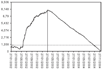
Figure 2. ICSS Statistic

Table 6. Repsol Series

*Significant at 5%

Given the significance of Q(10) in the first subsample, and that Q₂(10) does not reject the null, we tried to fit some model with significant parameters to this subsample and Taylor model, in Table 7, was selected. It has higher log-likelihood than the others but this is not remarkable because of the smaller sample size. Figure 3 presents Endesa, Repsol and subsample Repsol s estimated volatility. In this particular case, though in section II.B we questioned the Repsol s estimated volatility with all the sample under a change in unconditional variance, there are no big differences between Repsol s estimated volatility if we use all the sample information or if we estimate volatility in the subsample, even though conditional standard deviation estimated using Taylor model has a sawer pattern clearly. It is also quickly showed that Repsol s estimated volatility is quite similar to Endesa's one.

Table 7. Taylor Model

*These are estimated coefficients for Repsol s return series from January 3, 2002 to March 27, 2003.

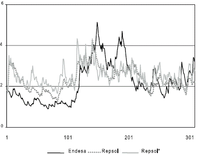
*Repsol's estimated volatility in subsample.

Figure 3. Endesa, Repsol and Repsol s Estimated Volatility

Conclusions

In order to analyze empirically financial time series of returns in the Spanish energy market, we have fitted a selection of different ARCH type models to the stocks returns series.

First, we have taken into account the presence of one outlier in two of our series, Gas Natural and Cepsa. We have treated the data for the outlier and explained what happened those days and which their effect in the analysis of both series is. We have corrected the series in order to avoid wrong conclusions. Also, we suspected the possibility of a change in the unconditional variance of Repsol s returns which could be very important in the estimation of Repsol s volatility. We have tested it using the ICSS algorithm proposed by Incláán and Tiao (1994). We have found the date of this change, and we have answered what happened on that day.

After estimating ARCH models, we have found that:
- In this particular case, taking into account the change in the unconditional variance of Repsol does not lead to big differences in the estimation of Repsol s volatility.
- The ARCH models used are able to capture a lot of regularities of our series. We have paid special attention in explaining the skewness present in the series.
- And finally, we have found that the electric market has been more volatile than gas and oil markets at the first until the middle part of the period analyzed, and we have seen how volatilities of these markets have been changing and lowering over time becoming similar and smaller at the end of the period. So, on average, electric market has been the most volatile market.

Furthermore, we were interested in looking for the relationship between the expected conditional stock return and its own conditional variance because there is a controversy in the literature on this subject. We used ARCH-M models and we found just two series with a significant and different relationship, negative for Enagas and positive for Cepsa, according to different positions in the literature.

Finally, this is a first approach to explain the behavior of the financial time series of the Spanish energy market. As this work is a univariate analysis, a multivariate analysis could be an interesting field of future research in order to identify relationships between stocks returns inside the market and their co-movement with other markets.

Notes

¹ Stock prices from the web www.bolsamadrid.es.

² Banco Bilbao Vizcaya Argentaria.

³ Banco Santander Central Hispano.

⁴ Jarque-Berastatisticforstandardizedresidualswasrejected.Bera statistic for standardized residuals was rejected.

⁵ These results were obtained from the estimation of r_t=v+ε_t though they do not appear in Table 2 in order to save space. For Cepsa we do not find significant v parameter in the models.

⁶ See Section II.B.

⁷ See Table 1.

⁸ Not in Tables.

Appendix

References

1. Black, Fischer (1976). Studies of Stock Price Volatility Changes, in Proceedings from the American Statistical Association, Business and Economic Statistics, American Statistical Association, pp. 177-181.        [ Links ]

2. Bollerslev, Tim (1986). Generalized Autoregressive Conditional Heteroskedasticity, Journal of Econometrics, Vol. 31, No. 3, pp. 307-327.        [ Links ]

3. Bollerslev, Tim (1987). A Conditional Heteroskedastic Time Series Model for Speculative Prices and Rates of Return, Review of Economics and Statistics, Vol. 69, No. 3, pp. 542-547.        [ Links ]

4. Bollerslev Tim and Wooldridge, Jeffrey M. (1992). Quasi Maximum Likelihood Estimation and Inference in Dynamic Models with Time Varying Covariances, Econometric Reviews, Vol. 11, No. 2, pp. 143-172.        [ Links ]

5. Bollerslev, Tim; Eengle, Robert F.; and Nnelson, Daniel B. (1994). ARCH Models. In Eeugle, F.F. and McFadden, D. (eds.), Handbook of Econometrics, Vol. 4. Amsterdam: North-Holland.        [ Links ]

6. Carnero, Maria A.; Peña, Daniel; and Rruiz, Esther (2004a). Persistence and Kurtosis in GARCH and Stochastic Volatility Models, Journal of Financial Econometrics, Vol. 2, No. 2, pp. 319-342.        [ Links ]

7. Carnero, Maria A.; Peña, Daniel; and Rruiz, Esther (2004b). Spurious and Hidden Volatility, Statistics and Econometrics Working Papers, No. ws042007, Universidad Carlos III, Madrid.        [ Links ]

8. campbell John Y. and Hentschel, Ludger (1992). No News is Good News. An Asymmetric Model of Changing Volatility in Stock Returns, Journal of Financial Economics, Vol. 31, pp. 281-318.        [ Links ]

9. Chan, Kakeung C.; Karolyi, G. Andrew; and Stulz, Rene M. (1992). Global Financial Markets and the Risk Premium on U.S. Equity, Journal of Financial Economics, Vol. 32, No. 2, pp. 137-167.        [ Links ]

10. Chen, Joseph; Hong, Harrison; and Stein, Jeremy (2001) Forecasting Crashes: Trading Volume, Past Returns and Conditional Skewness in Stock Prices, Journal of Financial Economics, Vol. 61, No. 3, pp. 345-381.        [ Links ]

11. Christie, Andrew (1982). The Stochastic Behavior of Common Stock Variances: Value, Leverage and Interest Rate Effects, Journal of Financial Economics, Vol. 10, No. 4, pp. 407-432.        [ Links ]

12. Diario Eexpansión (2003). Martes 11 marzo 2003, Año XVIII, No. 5052, pp. 4,10.        [ Links ]

13. Diario Eexpansión (2003). Viernes 28 marzo 2003, Año XVIII, No. 5067, pp. 12-14.        [ Links ]

14. Diario Eexpansión (2003). Sábado 27 septiembre 2003, Año XVIII, No. 5221, pp. 14.        [ Links ]

15. Ding, Zhuanxin; Granger, Clive W.J.; and Eengle, Robert F. (1993). A long memory property of stock market returns and a new model, Journal of Empirical Finance, Vol. 1, No. 1, pp. 83-106.        [ Links ]

16. Engle, Robert F. (1982). Autoregressive Conditional Heteroscedasticity with Estimates of the Variance of U.K. Inflation, Econometrica, Vol. 50, No. 4, pp. 987-1008.        [ Links ]

17. Engle, Robert F.; Llilien, David M.; and RrobBins, Russell P. (1987) Estimating Time Varying Risk Premia in the Term Structure: The ARCH-M Model, Econometrica, Vol. 55, No. 2, pp. 391-407.        [ Links ]

18. Engle, Robert F.; Iito, Takatoshi; and Llin, Wen-Lling (1990). Meteor Showers or Heat Waves? Heteroskedastic Intra Daily Volatility in the Foreign Exchange Market, Econometrica, Vol. 58, No. 3, pp. 525-542.        [ Links ]

19. Fama, Eugine F. (1965). The Behaviour of Stock Market Prices, Journal of Business, Vol. 38, No. 1, pp. 34-105.        [ Links ]

20. French, Kenneth R.; Schwert, G. William; and Stambaugh, Robert F. (1987). Expected Stock Returns and Volatility, Journal of Financial Economics, Vol. 19, No. 1, pp. 3-29.        [ Links ]

21. Ghysels, Eric; Harvey, Andrew; and Rrenault, Eric (1996). Stochastic Volatility. In Maddala, S. and Rrao, C. R. (eds.), Handbook of Statistics, Vol. 14, Amsterdam: North-Holland.        [ Links ]

22. Glosten, Lawrence R.; Jagannathan, Ravi; and Rrunkle, David (1993). On the Relation between the Expected Value and the Volatility of the Nominal Excess Return on Stocks, Journal of Finance, Vol. 48, No. 5, pp. 1779-1801.        [ Links ]

23. Higgins, Matthew L. and Bera, Anil K. (1992). A Class of Nonlinear ARCH Models, International Economic Review, Vol. 33, No.1, pp. 137-158.        [ Links ]

24. Hong, Harrison and Stein, Jeremy (2003). Differences of Opinion, Rational Arbitrage and Market Crashes, The Review of Financial Studies. Vol. 16, No. 2, pp. 487-525.        [ Links ]

25. Inclán, Carla and Tiao, George C. (1994). Use of Cumulative Sums of Squares for Retrospective Detection of Changes of Variance, Journal of the American Statistical Association, Vol. 89, No. 427, pp. 913-923.        [ Links ]

26. Jarque, Carlos M. and Bera, Anil K. (1987). A Test for Normality of Observations and Regression Residuals, International Statistical Review, Vol. 55, No. 2, pp. 163-172.        [ Links ]

27. Mandelbrot, Benoit (1963). The variation of Certain Speculative Prices, Journal of Business, Vol. 36, No. 4, pp. 394-419.        [ Links ]

28. McLleod, A.J. and Lli, W.K. (1983). Diagnostic Checking ARMA Time Series Models Using Squared-Residual Correlations, Journal of Time Series Analysis, Vol. 4, No. 4, pp. 269-273.        [ Links ]

29. Nelson, Daniel B. (1991). Conditional Heteroskedasticity in Asset Returns: A New Approach, Econometrica, Vol. 59, No. 2, pp. 347-370.        [ Links ]

30. Sentana, Enrique (1995). Quadratic ARCH Models, Review of Economic Studies, Vol. 62, No. 4, pp. 639-661.        [ Links ]

31. Schwert, G. William (1989). Why Does Stock Market Volatility Change Over Time, Journal of Finance, Vol. 44, No. 5, pp. 1115-1153.        [ Links ]

32. Taylor, Stephen (1986). Modeling Financial Time Series, Wiley and Sons: New York, NY.        [ Links ]

33. Zakoian, Jean-Michel. (1990). Threshold Heteroskedastic Models, Journal of Economic Dynamics and Control, Vol. 18, No. 5, pp. 931-955.        [ Links ]