The Environmental Kuznets Curve for Water Quality: An Analysis of its Appropriateness Using Unit Root and Cointegration Tests

 

La curva ambiental de Kuznets para el caso de la calidad del agua: un análisis de su pertinencia utilizando las pruebas de raíz unitaria y de cointegración

 

La courbe environnementale de Kuznets appliquée à la qualité de l'eau : Une analyse de sa pertinence en utilisant le test de racine unitaire et le test de cointégration.

 

 

*Catalina Granda;**Luis Guillermo Pérez; ***Juan Carlos Muñoz

*PhD student – Department of Economics, University of Connecticut. Candidate for Assistant Professor – Facultad de Ciencias Económicas, Universidad de Antioquia. Dirección electrónica: catalina.granda_carvajal@uconn.edu –cgranda@udea.edu.co. Dirección postal: University of Connecticut 341 Mansfield Road Unit 1063, Storrs, CT 06269, USA.

** Associate Professor – Facultad de Ciencias Económicas, Universidad de Antioquia. Dirección electrónica: lgperez@udea.edu.co. Dirección postal: A.A.1226, Medellín, Colombia.

*** Research Assistant – Centro de Estudios para Desarrollo Económico, Universidad de Los Andes. Dirección postal: jc.munoz135@uniandes.edu.co. Dirección postal: Carrera 1 Nº 18A–70, Bloque E Oficina 101, Bogotá, Colombia.

This paper received support from a grant by Comité para el Desarrollo de la Investigación at Universidad de Antioquia –CODI–.We would like to thank Mauricio Alviar Ramírez, Francisco Correa Restrepo and an anonymous referee for helpful comments on earlier versions of this article. Diana Restrepo Ochoa contributed to the analysis of some of the tests developed herein. Nonetheless, opinions stated throughout this paper are the sole responsibility of the authors.

 

–Introduction. –I. The Environmental Kuznets Curve. –II. Methodology and results. –Conclusions. –Appendix. –References

 

 

---

Resumen: La hipótesis de la Curva Ambiental de Kuznets sugiere la existencia una relación en forma de U invertida entre la degradación ambiental y el ingreso. Algunos economistas asumen que el crecimiento económico revertirá los impactos ambientales de las primeras etapas del desarrollo económico. No obstante, Perman y Stern (2003) argumentan que los métodos econométricos empleados en los primeros análisis de la EKC son inapropiados debido a las propiedades temporales de las series. Este artículo analiza la conformidad de la EKC para un panel de 46 países y 21 períodos mediante la implementación de pruebas de raíces unitarias y de cointegración a nivel individual y del panel. También se estima un Vector de Corrección de Errores. Los resultados obtenidos no corroboran la evidencia de una EKC común para el conjunto de países estudiados.

Palabras claves: Curva ambiental de Kuznets, crecimiento económico, pruebas de raíz unitaria y cointegración en panel de datos Clasificación JEL: Q53, Q56, C23

---

Abstract: The Environmental Kuznets Curve hypothesis suggests the existence of an inverted U–shaped relationship between environmental degradation and income. Several economists assume that the environmental impacts occurred during the first stages of the development process will be reverted as a result of economic growth. Yet Perman and Stern (2003) have argued that the econometric methods used in the earlier analysis of the EKC are inappropriate, given the time properties of the series. This article examines the appropriateness of the EKC for a panel of 46 countries and 21 periods by implementing individual and panel tests for unit roots and cointegration. An error correction model is also estimated. The results do not support evidence of a common EKC for the countries analyzed.

Keywords: Environmental Kuznets curve, economic growth, unit root and cointegration tests in panel data JEL Classification: Q53, Q56, C23

---

Résumé: L'hypothèse de la Courbe Environnementale de Kuznets (CEK) suggère l'existence d'une relation en U inversé entre la dégradation environnementale et le revenu. Plusieurs économistes estiment que les incidences négatives sur l'environnement qui sont produites pendant les premières étapes du processus de développement économique seront corrigées par les effets positifs de la croissance économique. Pourtant, Perman et Stern (2003) ont remis en cause la validité des méthodes économétriques employées dans les premières études de la CEK sur la base des propriétés des séries temporelles. Cet article examine la pertinence de la CEK en utilisant un panel de 46 pays et de 21 périodes et en conduisant des tests de racine unitaire et de cointégration aussi bien par pays que pour l.ensemble du panel. Un modèle à correction d'erreurs est également estimé. Les résultats ne soutiennent pas l.existence d'une CEK commune aux pays considérés dans le panel.

Mots clés : Courbe Environnementale de Kuznets, croissance économique, racine unitaire et test de cointégration dans des données de panel Classification JEL: Q53, Q56, C23

---

 

Introduction

The Environmental Kuznets Curve (EKC) hypothesis posits that there is an inverted U–shaped relation among various indicators of environmental degradation (pollution or resource depletion) and per capita income. Among the interpretations suggested for this hypothesis is that economic growth gives rise to changes in economic structure and technology, as well as to improvements in regulation and an enhanced environmental awareness that offset the impact of growth on the environment.

This hypothesis has brought back interest in the discussion about economic growth’s impact on the environment. In that sense, several economists assume that growth itself will lead to revert the environmental impacts made on the first stages of development and to environmental improvements in developed countries. Thus, they have stated that growth, far from being a threat for environmental quality, is necessary for its improvement and conservation.

Despite the EKC has faced considerable criticism on both theoretical and empirical grounds, it has become one of the ‘stylized facts’ of environmental and resource economics. However, cointegration analysis may prove useful to test the validity of such stylized facts when the data involved contain stochastic trends(Perman and Stern, 2003). The present study is focused on this alternative.

In order to do that, the EKC hypothesis is studied for Biochemical Oxygen Demand (BOD) with the aim to confirm whether that there is a long–run relationship between this water pollution indicator and income for every country. The panel studied includes 46 countries from 1980 to 2000. Besides per capita GNP, explanatory variables include a foreign trade intensity coefficient. Contrasts of unit roots and cointegration were individually applied to each country and to the panel data; afterwards, a number of models were adjusted with the introduction of deterministic trends and time dummy variables.

This paper is made up of four parts. In the first one, some potential explanatory factors for the EKC hypothesis are indicated, the main econometric aspects and the criticism, and studies related to BOD as well. Then the econometric approach used is described. The results obtained are analysed in the third part. To end, some conclusions and suggestions are outlined to feed further research.

 

I. The Environmental Kuznets Curve

The Environmental Kuznets Curve hypothesis was introduced in the early nineties with Grossman and Krueger’s work (1991) about the potential impacts of NAFTA, and with Shafik and Bandyopadhyay’s background study for the World Development Report in 1992. These studies showed the existence of an inverted U–shaped relationship between several pollutants and per capita income; that is, environmental quality initially deteriorates, but once countries reach a given income level, environmental degradation tends to decline. Panayotou (1993) called this relationship EKC because of its similarity with the relationship between income level and inequality in income distribution suggested by Simon Kuznets (1955). Since then, this term has become a reference point in the literature on growth and the environment.

In that sense, the EKC hypothesis has been useful to support the general proposition that economic growth will lead to remediate the environmental impacts of the first stages of development and to improve environmental quality in developed countries. Thus, some economists use it to support the statement that economic growth is a remedy to pollution and depletion of natural resources (Beckerman, 1992). Accordingly, they suggest fostering economic growth on the grounds that such an approach will drive the implementation of effective environmental policies (World Bank, 1992).

However, this assertion is preliminary due to the lack of unequivocal evidence regarding environmental degradation patterns throughout the determining factors of the EKC. Additionally, there are several aspects impeding to draw clear policy conclusions from this empirical hypothesis, economic development process, as well as to the lack of consensus on the which are mainly related to the EKC appropriateness for several kinds of environmental pressure and for all countries (individually and collectively) (de Bruyn and Heintz, 1999; Dinda, 2004).

 

A. Some suggested explanations

According to Barbier (1997), the explanations of the EKC have been focused on several underlying and dissimilar relations, including the effects of changes in the economic structure on the use of the environment, the links between the demand for environmental quality and income, and the types of environmental degradation and ecological processes. Some of the major explanations given to this empirical hypothesis are exposed in the following.

 

1. Scale, composition and technique effects

Economic growth affects the environmental quality through three different mechanisms, that is, the scale, composition and technique effects (Grossman and Krueger, 1991). The scale effect is reflected in a positive relation between environmental degradation and income; hence, environmental quality is expected to worsen as economic activity increases. However, with the increase in per capita income, changes in production mix may take place, leading an economy to less intense polluting sectors (for example, from industry to services). Similarly, growth may induce the adoption of technologies to enhance productive efficiency, in that they should use less polluting inputs per unit of output, or reduce polluting discharges per unit of input.¹ Under this scenario, environmental quality may suffer from degradation with income unless the scale effect is offset by a combination of the composition and the technique effects.

2. The impact of regulation

Grossman and Krueger (1995) interpret the EKC as a sign that environmental policy is carried out more effectively in a developed economy than in a developing one, as economic growth fosters demand for environmental quality and provides the resources to perform environmental protection measures (see also Panayotou, 1997). This explanation is further developed by Dasgupta et al. (2002), who indicate that evidence available suggests that regulation is the determining factor to explain pollution reduction as countries grow beyond the middle income status.

3. Foreign trade

Foreign trade causes contradictory impacts on the environment. As trade volume increases (especially exports), economy size increases, which damages environmental quality; however, trade could also lead to environmental improvements through the effects on the composition of economic activity and technology, mainly through consequences on the distribution of polluting industries.

Foreign trade benefits the decrease in production of pollution-intensive goods in one country as this production increases in the other(s). This composition effect is ascribed to two related hypotheses, namely, the displacement hypothesis and the pollution haven hypothesis. The displacement hypothesis refers to a situation where changes in the developed countries’ productive structure are not accompanied by equivalent changes in the consumption structure. In this case, the EKC would refer to the displacement of dirty industries towards developing economies (de Bruyn and Heintz, 1999).

On the other hand, the pollution haven hypothesis refers to the possibility that multinational firms, particularly those carrying out highly polluting activities, relocate their plants in countries having less stringent environmental regulations. According to this hypothesis, lower environmental standards should become a source of comparative advantage and, therefore, of changes in trade patterns (Stern et al., 1996). This hypothesis suggests primarily that highly regulated countries will ‘lose’ all the dirty industries that poor countries will get (Dinda, 2004).

However, if the validity of these hypotheses is proved, the estimated turning points of the EKC would be unrealistic since even with an increase in their income level, developing countries will not have the environmental rewards available to developed economies because of relocation (Stern, 1998).

B. Econometric aspects and criticisms

Most of the EKC analyses use panel data (Stern, 1998). For their estimation, a statistical reduced-form relation is employed, in which the chosen environmental degradation indicator is modelled as an inverted U-shaped function of per capita income, and thus the logarithm of the dependentvariable is associated to the square of the income log.² Using this methodology, the regression model assumes the following static form:

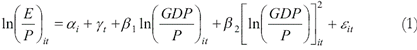
where E refers to environmental degradation, GDP represents the income level, P is the population level, and ln indicates natural logarithms. Variables are expressed across a series of countries (i = 1, …, N) and time periods (t = 1, …, T). The first two terms on the right hand side are the intercept parameters, which change among the various countries i and years t. They allow for specific effects across countries(αi ) and through time (γi ) with the aim to register common stochastic shocks. Random disturbances εit are assumed to be independent across countries, with variances that may differ across each of these.

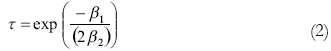
If the EKC hypothesis is met, then equation (1) has a common form, with β1> 0 and β2 < 0 for all i, and the income level at the turning point, where environmental quality is not affected by income, is given by

Comparing the estimated per capita income level associated to the turning point with the income levels observed in the data set can indicate whether the turning point falls in or out of the actual income range. This can shed light on the reliability of the EKC estimations (Barbier, 1997).

Most of the literature on the EKC has shown weak results from the econometric view. Concerning this, one of the more relevant aspects deals with the use of a reduced-form statistical relation, which eliminates the need of data on other variables that could affect the relation between per capita income and the pollution level, on the grounds that one equation captures the influence of income on technology, product mix and environmental policy, as well as the incidence that changes in these factors have on environmental pressure. The use of a reduced-form model has the advantage of providing a direct estimation of the net effect of income on environmental pressure (Correa Restrepo, 2004); however, it does not shed light on the nature of the estimated relation and, in particular, on coefficients analysis (Grossman and Krueger, 1995). Hence it is purely descriptive and does not allow observing the influence of growth on pollution patterns (de Bruyn et al., 1998; de Bruyn and Heintz, 1999; Panayotou, 1997).

Another controversial aspect has to do with the validity that estimated EKC relations on samples of countries may have for individual nations (de Bruyn et al., 1998). In that sense, some economists argue that the importance given to this hypothesis is based on the scarce attention that studies have paid to the statistical properties of the data, like serial correlation or stochastic trends in time series, and to the carrying out of model adjustment tests, such as the possibility of biases due to the omission of variables. Not long ago research reports having diagnosis statistics on series integration or cointegration among variables were quite reduced, and thus these are not clear as to what can be inferred on issues such as the significance of additional variables included in a reduced-form regression (e.g., economic openness indicators, among others) (Stern, 2004; Perman and Stern, 2003).

Perman and Stern (2003) find, using diagnosis tests for cointegration and unit roots in panel data relating sulphur emissions and income, that data are integrated in the time series dimension, that there are more than one cointegrating regression, and that these are not commonly of the EKC type for every country. These authors examine each individual country on the sample and find out that only some cointegrating relations estimated are consistent with the EKC hypothesis (typically, relations are U-shaped or monotonically rising in income). Based on these results, they suggest applying such diagnosis tests in studies related to other environmental indicators.

C. Empirical evidence and Biochemical Oxygen Demand

A number of models including explanatory variables other than income have been built with the aim to study the effect of underlying or approximate factors such as ‘political freedom’ (Torras and Boyce, 1998), economic structure (Panayotou, 1997; Suri and Chapman, 1998) or trade (Shafik and Bandyopadhyay, 1992; Suri and Chapman, 1998). Also, population density has been considered (Selden and Song, 1994) as well as lagged income (Grossman and Krueger, 1995), among others. The inclusion of these variables is intended
to improve the adjustment of estimations and to provide additional insights on pollutants behaviour as economies develop³ (de Bruyn and Heintz, 1999).

The literature on the EKC for water pollution, and particularly for pollution related to the oxygen regime (dissolved oxygen, Chemical Oxygen Demand, Biochemical Oxygen Demand), is scant and shows conflicting patterns. As for BOD, Grossman and Krueger (1995) and Correa Restrepo (2004) reportan EKC, but Shafik and Bandyopadhyay (1992) and Torras and Boyce (1998) find monotonically decreasing and N-shaped patterns, respectively. Despite the results are contradictory, all these studies are carried out following similar methodologies (regressions with panel data using ordinary or generalized least squares, per capita income measured in terms of purchasing power parity) and neglect the econometric diagnosis statistics.

The present study takes into account the criticisms mentioned in section I.A. and Perman and Stern’s (2003) suggestion concerning the estimation of a regression relating water pollution by BOD with income, including additionally a variable of foreign trade intensity. With this, we intend to contribute to a rigorous analysis of the validity of the EKC for various environmental degradation indicators.

 

II. Methodology and results

Static estimations were made for each country; panel data estimations with fixed and random effects; a dynamic error correction model for each country, which was additionally adjusted presuming the existence of a single EKC for all countries. Deterministic trends or time dummy variables were added to the earlier models. Prior to model estimation, unit root contrasts were made for each series employing individual and panel data tests, as well as individual and panel cointegration contrasts. Finally, the proposed models were validated. The software used is EViews 5.1.

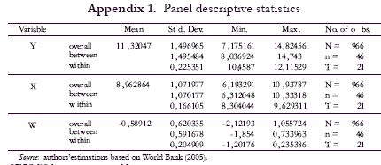
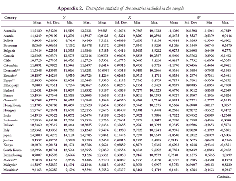
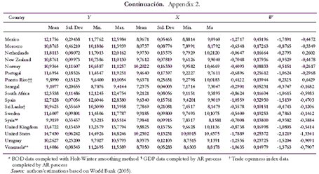
A. The data

The sample used was defined under data availability criteria. Annual data for 46 countries in the period 1980-2000 were considered (see descriptive statistics in Appendix 1). Still, the panel is unbalanced as some data are missing (not more than two per time series), an unbalance corrected using smoothing methodologies.⁴ The countries considered are classified as high, middle and low income, as we wanted to comprise a heterogeneous group,⁵ which is in accordance with the estimation method used. The main aspects of the variables used in the model are explained as follows.

1. The dependent variable

Biochemical Oxygen Demand (BOD) is the water pollution indicator most used by regulatory agencies.⁶ It measures the oxygen dissolved that micro-organisms require for the decomposition process of organic matter in water bodies.⁷ We use the BOD series featured on the World Development Indicators (World Bank, 2005), which refers to polluting emissions (in kg/day).

2. The explanatory variables

–Gross Domestic Product per capita

As indicated before, income is the (more) relevant explanatory variable in the EKC hypothesis. This variable is represented by per capita Gross Domestic Product in terms of purchasing power parity (PPP). The series were taken from the World Development Indicators published in 2005 (World Bank 2005).

–Foreign trade intensity

Trade intensity, defined as the ratio of exports plus imports and GDP, is a coefficient used to measure openness to foreign trade. Like the previous variables, the data were taken from the World Development Indicators published in 2005 (World Bank, 2005). It is worth noting that even though this indicator has been quite used in the literature on the EKC that considers foreign trade (Grossman and Krueger, 1991; Shafik and Bandyopadhyay, 1992), it has been bly criticized as it gives an account of trade policy orientation rather than of observed trade (Stern, 1998; Suri and Chapman, 1998).

As the values of the variables to be used are all positive and given the general functional specification of the EKC (equation (1)), we take the logarithm of the various variables. For the sake of simplicity, the natural logs of BOD, GDP per capita and foreign trade intensity are denoted as Y, X and W, respectively. The square of X is called Z.

B. Econometric Procedures and Analysis of Results

1. Unit root tests

The implementation of unit root tests for both each series and the panel data is mainly due to the proven fact that individual tests have low power when they are applied to short series, while panel tests increase the power of contrasts (Perman and Stern, 1999). However, individual tests are useful to support the results obtained with panel tests.

–Individual unit root tests

Dickey-Fuller (ADF), Phillips-Perron (PP) and Kwiatowski et al. (KPSS) tests were applied. For that, the optimal lag length was chosen attending to the Schwarz’s information criterion, as well as a consistent estimator of the varianceusing the Newey-West method. Table 1 shows the number of countries for which the three contrasts used allow to conclude that the series are stationary at five and ten percent levels of significance.

When a trend is not included in the contrast, ADF and PP tests show similar results: most series have a unit root. On average, the null hypothesis has been rejected only for two countries under all variables. Following the same specification, the null hypothesis of stationarity is more often not rejected on the KPSS test (for the natural log of BOD, the stationarity hypothesis can not be rejected in 17 countries). When the tests include an individual trend, ADF and PP results show more rejections of the unit root null hypothesis (four on average) compared to the results of the same tests with no trend. The KPSS test shows a higher number of non rejections for the null hypothesis of stationarity.

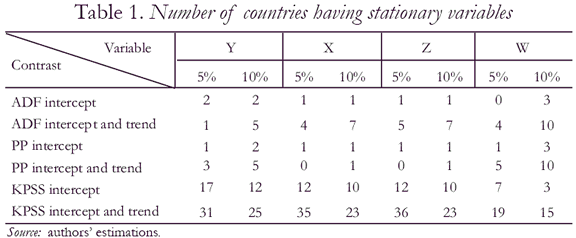
In sum, the unit root individual tests allow us to state that most series corresponding to the various countries in the sample are integrated of order one−i.e. I(1). Note that, when analyzing the series in first differences, these proved to be stationary.

–Panel unit root tests

Two approaches are employed: common (Levin and Lin; Hadri) and individual (Im, Pesaran and Shin). The individual approach considers heterogeneity among the panel individuals, while the common approach does not. Following Perman and Stern (2003), we call Levin and Lin’s statistic panel statistic, and Im, Pesaran and Shin`s statistic group statistic. Hadri’s test statistic is considered separately. Table 2 shows a clear trend on all contrasts to not rejecting the hypothesis of existence of stochastic trends in all series, except for X and Z, for which the non-trended panel statistic allows rejecting the null hypothesis.

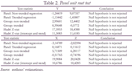
In Hadri’s stationarity test, the null hypothesis is rejected for all series, which shows that the series analyzed have a unit root. Thus, there is b evidence that all the series included in the panel are integrated of order one. Individual series analysis, besides, helps to validate the insight on the existence of a unit root in the panel.

2. Cointegration tests

The previous results make further tests required in order to find a long-run relation connecting the series, that is, to ensure that we are not in the presence of a spurious relation.

–Individual cointegration tests

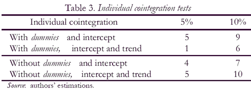
The Engle and Granger procedure is followed. The analysis is applied on two groups of models. In the first group, we take the variables in deviations from their transversal means or time dummies, while these are not contained in the second group. Perman and Stern (1999) indicate that these dummies can be used as proxies of common effects on time. Their inclusion is meant to eliminate
dependence between country-related errors.

Table 3 shows the results obtained for each of the estimated models. Individually, there is no b evidence supporting the existence of cointegration, as statistically speaking the higher number of significant long-run relations is ten. Only two countries (Bolivia and Sri Lanka) show evidence of cointegration in all the four models at ten percent level of significance.

In the following section, the results from some panel cointegration tests are analyzed.

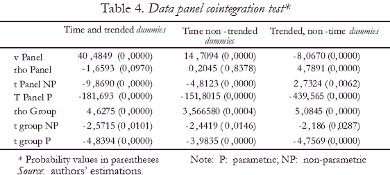
–Panel cointegration tests

Several approaches to prove the existence of a potential cointegration relation have emerged recently. These approaches are based on the traditional ones to individual cointegration. In this paper, we follow Pedroni’s (1999) approach, as he takes up again the residuals-based conceptualisation posited by Engle and Granger, and formulates seven test statistics that allow assuming heterogeneity in the panel. This author proposes two approaches to contrast cointegration: panel and group statistics. The panel statistics are made on the within dimension, that is, fixed effects are presupposed. The group statistics are made on the between dimension, that is to say, the mean for each individual in the panel is obtained before adding on the N dimension.

The results from Pedroni’s cointegration tests are shown in table 4. It can be seen that the various tests allow rejecting the no-cointegration null hypothesis. This result is important as, unlike the individual cointegration tests, it shows a long-run relation among the variables. Note that the no-cointegration hypothesis is not rejected only in the test with the time non-trended dummies rho panel statistic. This is evidence supporting the heterogeneity present among the panel individuals.

These results beg some questions regarding the existence of a long-run relation of the EKC type common to all countries, which will be discussed in the following section.

3. Estimation of models

The econometric work is primarily based on the estimation of a dynamic model. However, various static models were adjusted. The static model for each country has the form

Where i =1, 2,…, 46 and t = 1980, 1981, …, 2000. Each transversal unit/ variable is related to its respective parameter. This model was adjusted with a deterministic trend or with time dummies. The assumptions on the disturbance term are the classical ones. The methodology used was ordinary least squares. Fixed and random effects models are given by

Where the disturbance term has the form εit=φi+ηit. It is assumed that ηit is not correlated with the explanatory variables. φi is called the country’s individual effect i, constant in time. In the fixed effects model φi is considered a parameter, while it is treated as a random variable in the random effects model. Under the classical assumptions, the model with fixed effects is estimated by ordinary least squares, whereas generalized least squares is used for estimating the model with random effects.

Given that the variables are integrated of order one, previous static relations being spurious is at risk. Similarly, the model residuals are very likely to be correlated even though estimations are consistent but biased. The estimations can be improved using error-correction dynamic models wherein, assuming that the variables are cointegrated, classical inference is valid. Moreover, since lags are introduced in the regressors, problems such as correlation of residuals may possibly be amended. The error-correction model is as follows:

A single lag is used for all variables, as otherwise the number of parameters would be too large; also, the model is adequate in this situation. This is a very general model, as all the parameters associated to the distinct variables are different for each transversal section. αi is the error-correction coefficient related to country i, and reports on the speed of adjustment towards equilibrium. To
have a long-run relation, it has to be the case that −1< αi < 0 .

μi is the fixed effects parameter, which varies among the different countries. ηt is the intercept related to year t. With ηt , which implies introducing time dummy variables in the model, we seek to control the common effect associated to time; thus, by taking into account the presence of μi and the lags in the model, we can assume that the disturbance terms εit are independently distributed through time and across countries, with zero mean and constant variance per country. We can add a deterministic trend associated to each country to the previous model.

Among the existing possibilities, two models were selected. The first model includes a deterministic trend within the long-run relation, but no time dummies; in the second one, the roles of those variables are interchanged. The second model was estimated after extracting from each datum the transversal mean of the corresponding year. The estimation of these models, called nonrestricted models, allows studying in a clearer statistical way whether the EKC actually exists for every country. Also, it is possible to estimate the average of each long-run parameter from the average of the corresponding estimates, and to calculate a common estimate of the turning point for all countries based on that information.⁸

One way to study the EKC hypothesis is to subject the previous model, in both versions, to the restriction β1i = β1, β2i = β2, β3i = β3, i = 1, 2, …, n, called a restricted model, and to analyze whether data do not allow to reject such a restriction. Non rejection of the null hypothesis implies that there exists a single long-run relation and, therefore, it would validate the EKC hypothesis. The estimation methodology used was weighted least squares, as it enables one to take into account the likely heteroscedasticity of the disturbance term in each country. The basis on which to contrast the EKC hypothesis is the likelihood ratio, asymptotically chi-square distributed with q degrees of freedom, where q is equal to the number of restrictions.

The static models for each country were adjusted so that one would be trended and the other would have time but not trended dummy variables. These models show b correlation problems in residuals (high R-square and Durbin-Watson statistic close to zero). In the trended model, 26 countriesmeet the EKC hypothesis, while in the other case the models corroborating this hypothesis amount to 33. Both fixed and random effects models meet the EKC assumptions, but as the static models, they are not statistically valid.

In tables 5 and 6, the main results for the dynamic models are presented. At the individual level, it can be noticed that there are 30 countries that verify the EKC hypothesis, which is similar to the results obtained for the static models. However, these results are invalid, because only 4 countries in the non-dummies trended model meet all of the necessary hypotheses (speed of adjustment between -1 and 0 and statistically significant, statistically significant parameters with appropriate signs). Also, we may conclude that for 11 countries, the longrun relation is valid. In the model with dummies, 3 countries corroborate all hypotheses, and 4 show cointegration.

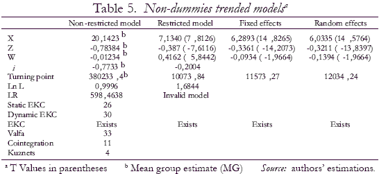
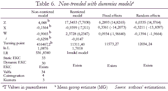
The null hypothesis of existence of a unique EKC for all 46 countries in both types of models is rejected with a probability value of zero. This allows us to assert that, for these data, parameters are not homogeneous in the long run and, therefore, the EKC does not exist for this set of countries. Also, it can be inferred that the static results, which have traditionally shown fixed or random effects, are spurious; that is, the results of the two last columns in tables 5 and 6 do not have any statistical validity.

The results obtained for the income level associated to the turning point in the restricted models and in the estimations with random and fixed effects are convincing because of their relative similarity and because they are located within the set of values of per capita income for all of the countries. However, individually, income associated to the turning points in the four models mentioned falls in the range of income for six nations only. As we have said, these conclusions are void of statistical validity.

 

Conclusions

 

The EKC hypothesis posits the existence of a U-shaped relation between environmental degradation and per capita income. This hypothesis has been criticized because several authors have assumed that it entails economic growth as a precondition to implement environmental effective policies, and thus to revert the impacts caused to the environment during the first stages of development (Beckerman, 1992; World Bank, 1992). Besides, the importance given to the EKC hypothesis is supported by the limited or void attention given to the econometric diagnosis statistics that studies on the topic usually exhibit (Stern, 2004). In particular, it is believed that what has been traditionally done (estimations with panel data on static models with random or fixed effects) poses specification problems due to the presence of first-order integrated series; also, because homogeneity is assumed in the parameters for different countries, which can be incorrect.

The results obtained in this study show evidence that all the series exhibit stochastic trends both on the individual and on the panel level. As for cointegration, it does not appear among the series for most of the countries taken individually, though it does appear for the panel data. Nonetheless, the different estimates show that, even if there is a long-run relation among BOD, per capita GDP (linear and squared) and foreign trade intensity, this is not an EKC for the set of nations considered.

Even more, models under restrictions and estimates with random and fixed effects are not statistically valid. This is remarkable given the relative consistency that these estimates show in favour of the EKC hypothesis and because of theincome levels associated to the turning points obtained. However, individual results support conceptual criticism on the EKC hypothesis since most of the countries have not yet achieved the per capita income levels that allow them improvements in water quality, which contributes to worsen global environmental degradation (Stern et al., 1996; Arrow et al., 1995).

Following the explanations to the EKC posited on the literature, and since such hypothesis reports a relation between the income level and environmental pressure exclusively, an additional variable has been tried in order to consider the incidence of foreign trade. But such a variable, a foreign trade intensity coefficient, has turned out to be not very significant from the statistic perspective and with little relevance for the analysis. This rather confirms the criticism that the inclusion of this variable has received in some studies on the EKC (Stern, 1998; Suri and Chapman, 1998), and raises the need to include other trade indicators capable of giving an account of relocation of polluting activities. This consideration can be generalized as these indicators allow considering other underlying or proximate factors, thereby providing sound explanations about changes in water quality as economic development unfolds.

The results obtained match up Perman and Stern’s (2003) on sulphur dioxide (an indicator of atmospheric pollution). Then it can be said that, to make appropriate analyses of the EKC hypothesis, unit root and cointegration contrasts should be applied at the individual and panel levels. In this sense, we suggest to continue the use of such procedure when addressing relations between economic growth and environmental quality.

Yet it should be noted that the lack of data, mainly for the time interval considered, plays down power to the unit root and cointegration tests presented here. Similarly, hypothesis tests on unit roots and panel cointegration continue to be incipient. Another limitation has to do with the lack of randomness in the selection of countries comprising the panel, so inferences can not be made on the basis of actual estimations to countries not included in the sample.

In brief, theoretical and econometric criticisms on the EKC, partly supported by the results achieved throughout this study, suggest the need to reformulate the relation between economic growth and water degradation and, in general, between growth and environmental quality. It is obvious that the EKC may be configured from innumerable possible results derived from economic growth. Therefore, instead of ascribing the EKC to a single factor, appropriate attention should be paid to the other elements that make up the system economy-environment. In this sense, further research needs to give priority to the identification of the more relevant aspects when explaining such a relation, since this would be the only way to formulate policies able to influence it.

 

 

References

1. Alviar Ramírez, Mauricio; Granda Carvajal, Catalina; Pérez Puerta, Luis Guillermo; Muñoz Mora, Juan Carlos y Restrepo Ochoa, Diana Constanza (2006). Determinantes de la Curva Ambiental de Kuznets para la Calidad del Agua: un análisis empírico, Informe de investigación, Medellín, Universidad de Antioquia-Centro de Investigaciones Económicas.        [ Links ]

2. Arrow, Kenneth; Bolin, Bert; Costanza, Robert; Dasgupta, Partha; Folke, Carl; Holling, C. S.; Jansson, Bengt-Owe; Levin, Simon; Mäler, Karl- Göran; Perrings, Charles and Pimentel, David (1995). ''Economic Growth, Carrying Capacity, and the Environment'', Science, Vol. 268, 28 April, pp. 520-521.        [ Links ]

3. Baltag i, Badi (2001). Econometric analysis of panel data, Second edition, Chichester, John Wiley & Sons.        [ Links ]

4. Barbier, Edward B. (1997). ''Introduction to the environmental Kuznets curve special issue'', Environment and Development Economics, Vol. 2, No. 4, March, pp. 369-381.        [ Links ]

5. Beckerman, Wilfred (1992). ''Economic growth and the environment: whose growth? Whose environment?'', World Development, Vol. 20, No. 4, April, pp. 481-496.        [ Links ]

6. De Bruyn, Sander M. and Heintz, Roebijn J. (1999). ''The environmental Kuznets curve hypothesis''; in van den Bergh, Jeroen C. J. M (ed.), Handbook of Environmental and Resource Economics, Cheltenham and Northampton, Edward Elgar.        [ Links ]

7. De Bruyn, S. M.; van den Bergh, J. C. J. M. and Opschoor, J. B. (1998). ''Economic growth and emissions: reconsidering the empirical basis of environmental Kuznets curves'', Ecological Economics, Vol. 25, No. 2, May, pp. 161-175.        [ Links ]

8. Correa Restrepo, Francisco (2004). Crecimiento económico, desigualdad social y medio ambiente: evidencia empírica internacional, Tesis de Maestría, Medellín, Universidad Nacional de Colombia.        [ Links ]

9. Dasgupta, Susmita; Lap lante, Benoit; Wang, Hua and Wheeler, David (2002). ''Confronting the Environmental Kuznets Curve'', Journal of Economic Perspectives, Vol. 16, No. 1, Winter, pp.147-168.        [ Links ]

10. Dinda, Soumyananda (2004). ''Environmental Kuznets Curve Hypothesis: A Survey'', Ecological Economics, Vol. 49, No. 4, August, pp. 431-455.         [ Links ]

11. Enders, Walter (2004). Applied econometric time series, Second edition, Chichester, John Wiley & Sons.        [ Links ]

12. Grossman, Gene M. and Krueger, Alan B. (1995). ''Economic Growth and the Environment'', Quarterly Journal of Economics, Vol. 110, No. 2, May, pp. 353- 377.        [ Links ]

13. Grossman, Gene M. and Krueger, Alan B. (1991). ''Environmental Impacts of a North American Free Trade Agreement'', NBER Working Paper, No. 3914, Cambridge, National Bureau of Economic Research.         [ Links ]

14. Kuznets, Simon (1955). ''Economic growth and income inequality'', American Economic Review, Vol. 45, No. 1, pp. 1-28.        [ Links ]

15. Mahía, Ramón (2000). ''Análisis de estacionariedad con datos de panel: una ilustración para los tipos de cambio, precios y mantenimiento de la PPA en Latinoamérica'', Mimeo, Instituto L. R. Klein, junio.        [ Links ]

16. Metca lf & Eddy (1995). Ingeniería de aguas residuales: tratamiento, vertido y reutilización, Vol. 2, Third edition, McGraw Hill Interamericana.        [ Links ]

17. Panayotou, Theodore (1997). ''Demystifying the environmental Kuznets curve: turning a black box into a policy tool'', Environment and Development Economics, Vol. 2, No. 4, March, pp. 465-484.        [ Links ]

18. Panayotou, Theodore (1993). ''Empirical tests and policy analysis of environmental degradation at different stages of economic development'', International Labour Office Discussion Paper 1, Geneva.        [ Links ]

19. Pedroni, Peter (2004). ''Panel Cointegration: Asymptotic and Finite Sample Properties of Pooled Time Series Tests with an Application to the PPP Hypothesis'', Econometric Theory, Vol. 20, No. 3, June, pp. 597-625.        [ Links ]

20. Pedroni, Peter (1999). ''Critical values for cointegration tests in heterogeneous panels with multiple regressors'', Oxford Bulletin of Economics and Statistics, Vol. 61, Special issue, November, pp. 653-670.        [ Links ]

21. Perman, Roger and Stern, David I. (2003). ''Evidence from panel unit root and cointegration tests that the Environmental Kuznets Curve does not exist'', Australian Journal of Agricultural and Resource Economics, Vol. 47, No. 3, September, pp. 325-347.        [ Links ]

22. Perman, Roger and Stern, David I. (1999). ''The Environmental Kuznets Curve: Implications of Non-Stationarity'', Mimeo, June.        [ Links ]

23. Pesaran, M. Hashem and Smith, Ron (1995). ''Estimating long-run relationships from dynamic heterogeneous panels'', Journal of Econometrics, Vol. 68, No. 1, July, pp. 79-773.        [ Links ]

24. Pesaran, M. Hashem; Shin, Yongcheol and Smith, Ron (1998). ''Pooled Mean Group Estimation of Dynamic Heterogeneous Panels'', Mimeo, University of Cambridge.        [ Links ]

25. Selden, T. and Song, D. (1994). ''Environmental quality and development: is there a Kuznets Curve for air pollution emissions?'', Journal of Environmental Economics and Management, Vol. 27, No. 2, September, pp. 147-162.        [ Links ]

26. Shaf ik, Nemat (1994). ''Economic development and environmental quality: an econometric analysis'', Oxford Economic Papers, Vol. 46, Special Issue on Environmental Economics, October, pp. 757-773.        [ Links ]

27. Shaf ik, N. and Bandyopa dhyay, S. (1992). ''Economic growth and environmental quality: time series and cross-country evidence'', Background paper for the World Development Report, Washington, D.C., The World Bank.        [ Links ]

28. Stern, David I. (2004). ''The Rise and Fall of the Environmental Kuznets Curve'', World Development, Vol. 32, No. 8, August, pp. 1419-1439.         [ Links ]

29. Stern, David I. (1998). ''Progress on the environmental Kuznets curve?'', Environment and Development Economics, Vol. 3, No. 2, March, pp. 173-196.        [ Links ]

30. Stern, David I.; Common, Michael S. and Barbier, Edward B. (1996) ''Economic Growth and Environmental Degradation: The Environmental Kuznets Curve and Sustainable Development'', World Development, Vol. 24, No. 7, July, pp. 1151-1160.        [ Links ]

31. Suri, Vivek and Chap man, Duane (1998). ''Economic growth, trade and energy: implications for the environmental Kuznets curve'', Ecological Economics, Vol. 25, No. 2, May, pp. 195-208.        [ Links ]

32. Torras, Mariano and Boyce, James K. (1998). ''Income, inequality, and pollution: a reassessment of the environmental Kuznets Curve'', Ecological Economics, Vol. 25, No. 2, May, pp. 147-160.        [ Links ]

33. World Bank (2005). World Development Report, Washington, D.C. (CD-ROM).        [ Links ]

34. World Bank (1992). World Development Report, Washington, D.C.        [ Links ]

 

 

Primera versión recibida en junio de 2008; versión final aceptada en agosto de 2008

 

Notas

 

1 The adoption of technologies may also be the result of changes in underlying variables related to economic development, such as more stringent environmental regulation and/or higher educational level of the population. In a similar way, it may be directed by the market (partly fostered by the benefits of environmental conservation).

2 Note that this functional specification does not allow for incorporation of null or negative values of the environmental degradation indicators.

3 Compared to the values estimated without their inclusion, such variables capture some part of the polluting effects associated to income and, as a consequence, can alter the turning points.

4 The BOD series were corrected with the non-seasonal Holt-Winter smoothing method, while the series for economic openness and per capita GDP were corrected through autoregressive processes.

5 For each country’s descriptive statistics, see Appendix 2. We thank a referee for suggesting us this point.

6 As a matter of fact, developing countries have traditionally started industrial pollution control programs by regulating emissions of this pollutant.

7 There are other indicators of water pollution by organic compounds. One of them is Chemical Oxygen Demand (COD), which measures the dissolved oxygen required by a chemical oxidant to decompose the organic material contained both in natural and waste waters.

8 Pesaran and Smith (1995) show that the estimator obtained using this procedure (mean group estimator, MG) consistently estimates the parameter average.

 

Appendix