


Services on Demand
Journal
Article
 English (pdf)
 Article in xml format
 Article references
 Send this article by e-mail
Indicators
-
 Cited by SciELO
 -
 Access statistics
Related links
-
 Cited by Google
 -
 Similars in
SciELO
Similars in
SciELO -
 Similars in Google
Share

 Permalink
Lecturas de Economía
Print version ISSN 0120-2596
Lect. Econ. no.79 Medellín July/Dec. 2013
ARTÍCULOS
Gold prices: Analyzing its cyclical behavior
Los precios del oro: Análisis de su comportamiento cíclico
Le prix de l'or : Une analyse de son comportement cyclique
Martha Gutiérrez1, Giovanni Franco2, Carlos Campuzano3
1 Energy analyst, Negotiation of Energy Solutions, ISAGEN S.A. E.S.P., Cr. 30 # 10c-280 Medellín - Colombia. Email: mgutierrez@isagen.com.co.
2 School of Materials Engineering, National University of Colombia. Ph.D(c), Mine Planning Group Research, Carrera 80 No. 65-223 Medellín – Colombia. Email: gfranco@unal.edu.co.
3 School of Materials Engineering, Mine Planning Group Research, National University of Colombia, Carrera 80 No. 65-223 Medellín – Colombia. Email: cacampuz@unal.edu.co.
–Introduction. –I. Fixing of Gold Prices. –II. Conceptual Framework. –III. Analysis of the DJIA/GF ratio. –IV. Discussion of Results. –Conclusions. –References.
Primera versión recibida el 11 de octubre de 2012; versión final aceptada el 16 de septiembre de 2013
ABSTRACT
Gold is a commodity that is seen as a safe haven when a financial crisis strikes, but when stock markets are prosperous, these are more attractive investment alternatives, and so the gold cycle goes on and on. The DJIA/GF (Dow Jones Industrial Average and Gold Fix ratio) is chosen to establish the evolution of gold prices in relation to the NYSE. This paper has two goals: to prove that the DJIA/GF ratio is strongly cyclical by using Fourier analysis and to set a predictive neural networks model to forecast the behavior of this ratio during 2011-2020. To this end, business cycle events like the Great Depression along with the 1970s crisis, and the 1950s boom along with the world economic recovery of the 1990s are contrasted in light of the mentioned ratio. Gold prices are found to evolve cyclically with a dominant period of 37 years and are mainly affected by energy prices, financial markets and macroeconomic indicators.
Key words: Gold cycle, DJIA/GF ratio, Fourier analysis, neural network forecast.
JEL classification: L72, Q02, F47, F44.
RESUMEN
El oro es un bien básico que se ve como refugio cuando una crisis financiera acontece; pero cuando los mercados de valores son prósperos, las acciones son una alternativa más atractiva, y así se da el ciclo del oro. El DJIA/GF (relación entre el Índice Industrial Dow Jones y el precio del oro) permite establecer la evolución de los precios del oro en relación con el NYSE. Este trabajo tiene dos objetivos: demostrar que la relación DJIA/ GF es fuertemente cíclica usando análisis de Fourier, y establecer un modelo de redes neuronales para predecir el comportamiento de esta relación durante 2011-2020. Para ello, eventos económicos cíclicos como la Gran Depresión junto con la crisis de los años 70, y el auge de los años 50 junto con la recuperación de los 90, se contrastan a la luz de la relación DJIA/GF. Se encuentra que los precios del oro evolucionan cíclicamente con un periodo dominante de 37 años y están afectados principalmente por los precios de los energéticos, los mercados financieros e indicadores macroeconómicos.
Palabras clave: Ciclo del oro, relación DJIA/GF, análisis de Fourier, pronóstico de red neuronal.
Clasificación JEL: L72, Q02, F47, F44.
RÉSUMÉ
L'or est une marchandise qui est considéré étant un refuge en cas de crise financière, mais lorsque les marchés boursiers sont en plein essor, les actions sont une alternative plus intéressante. Ceci donne naissance au cycle de l'or. Le ratio ente l'indice industriel Dow Jones et le prix de l'or (DJIA/GF) montre l'évolution du prix de l'or par rapport à la NYSE (New York Stock Exchange). Cet article a deux objectifs: premièrement, il s'agit de démontrer que le ratio DJIA/GF est très cyclique lorsqu'on utilise l'analyse de Fourier et, deuxièmement, il s'agit d'établir un modèle de réseau neuronal pour prédire le comportement de ce ratio entre 2011 et 2020. Pour ce faire, les événements économiques comme la Grande Dépression, la crise des années 70, le boom des années 50 ou bien la reprise des années 90, sont contrastés à la lumière du ratio DJIA/GF. Nous constatons que les prix de l'or évoluent de manière cyclique avec une période dominante de 37 ans et ceux-ci sont essentiellement influencés par les prix de l'énergie, par les marchés financiers et par les agrégats macroéconomiques.
Mots clés: cycle de l'or, ratio DJIA/GF, analyse de Fourier, prévisions à travers un réseau neuronal.
Classification JEL: L72, Q02, F47, F44.
Introducción
For centuries, gold has had the interesting characteristic of being a commodity, i.e., it is money and product at the same time. Because it has always been a universally-accepted product that is itself a store of value, the vast majority of countries around the world took the metal as a common denominator of all economic transactions (Craig, Fisher & Spencer, 1995; Lothian, 2002; Smith & Shubik, 2011). Furthermore, gold has continually met all the requirements that a good commodity should: it is durable (it is stainless, it is an ''inert'' metal), it has a high market value, it is portable and it is homogeneous (i.e. it has always been a good with advantages over any other media of exchange). Today gold takes the form of a store of value held in the inventories of central banks around the world as a reserve that keeps its purchasing power. Gold can act as a stabilizing force in the financial system, reducing losses in the face of negative swings in the market (Baur & Mcdermott, 2010).
Gold prices are basically affected by three factors: the proved reserves of gold and energy prices, financial markets and macroeconomic factors (Lili & Chengmei, 2013). Particular events that have effect over gold prices have to do with one of the three named groups; for instance, the global financial market is under uncertainty in the sense of the trust of investors on it, the 2008 financial crisis in the USA is an example of distrust on being a company shareholder, and it can be verified how the price of gold rose rapidly during the following years until a slight recovery in the financial market took place (Kitco, 2013; Mollick & Assefa, 2013; Shachmurove, 2011). Gold reserves add to the supply of the metal to the market, and the price is going to be directly affected by how much gold central banks store and emit to the global market (Aizenman & Inoue, 2013). The mining reserves add their influence too, because the gold market is speculative, and while mines produce more or less gold and augment the circulating supply around the world, its price is affected. Global macroeconomic factors also have a direct effect on gold prices, like inflation, CPI, unemployment rates, stock index returns, treasury bond prices, interest rates, among others (Christie–David, Chaudhry, & Koch, 2000; Mollick & Assefa, 2013).
This paper aims to unveil the gold cycle in relation to the stock markets, which is very well measured by the Dow Jones industrial Average and Gold Fix ratio (DJIA/GF). To this end, we analyze the business cycles observed throughout the XX century and the elapsed years of the XXI century in light of the DJIA/GF ups and downs; then, a Fourier analysis allows one to have a deep understanding of the strongly cyclical behavior of the DJIA/GF ratio; and, finally, we build a predictive model based on artificial intelligence methodologies, i.e., neural networks in this case of study.
A crucial fact has to be faced, gold prices are too volatile, that is, they have a high variance to be predicted with the desired precision for investors like mining companies, central banks, and all the speculative agents of this market, which makes it a high risk one also (Shafiee & Topal, 2010); in other words, any prediction of its nominal or real price has a very high level of uncertainty of being even accurate. Many models for predicting gold prices have been built: the Markov chain combination method, the BP neural network model, Grey Markoff model, among others for the Chinese case of study. There are many others, like the Factor-augmented VAR model (Lili & Chengmei, 2013), which the very authors acknowledge is a rough one to predict gold prices. Most of the models propose linear or non-linear relationships between multiple variables and the gold price. The fact that macroeconomic cycles affect gold prices is ignored, or partially taken into account, when this fact is of great importance in order to predict trends in gold prices with good accuracy, and also to understand the current circumstances about the matter. The latter is supported on the fact that the price of gold relates in a direct proportional way to gold reserves and prices of energy products, while it relates in a converse proportional way to financial market indexes and global macroeconomic indicators (Lili & Chengmei, 2013), and on studies about gold bubble prices and financial crisis, to analyze the Dow Jones Industrial Average divided by the Gold Fix, i.e., the DJIA/GF ratio (Prechter, 2009), by using data since 1900 to 2010. As the DJIA is a financial variable that is reported daily and affects gold price conversely, it was suspected to be found some sort of cyclical component in it, and it was found.
The DJIA/GF ratio has a strong cyclical component, which was proved by means of the Fourier Series, which is of help in decomposing the named into harmonic terms, so as to allow the corresponding Frequency Analysis to be performed (Kreizig, 2006). This methodology was of help to determine a strong cyclical component in the time series of the DJIA/GF ratio, represented by its third harmonic, which has a noticeable dominant magnitude in comparison to the rest. Besides, the distance in time between minimums and maximums is approximately constant and is between 34 and 37 years, being 37 years the period of the third harmonic of the named series. After proving that this time series has a strong cyclical behavior through time, a predictive model is built by means of Neural Networks. This procedure proved to be very accurate for predicting the already known points, and because of its ability to recognize complex time series behaviors like the one studied in this paper. Thus, it was of great support for predicting future values of the DJIA/GF time series until 2020. Both of the models coincide in telling the trends of the DJIA/GF time series, which empowers a simple model to be a good basis for understanding a very volatile market, like gold's, in relation with the stock market, which is represented by the DJIA.
In the first section of this paper, it is studied the gold fixing evolution, and introduced the Dow Gold ratio, or DJIA/GF, as a tool to study the gold cycle, to face the volatile behavior of gold prices alone. The second section discusses the influential factors on gold prices with more depth. The third section presents a theoretical framework of the models used in this paper to study the DJIA/GF ratio, i.e., Fourier series and Neural Networks. The following section is the core of this paper, a Fourier Analysis is performed over the DJIA/GF to prove it is cyclical with a dominant period of 37 years, though it is not useful for making punctual nor even approximate predictions; then it is all about the making of a predictive model for the DJIA/GF ratio valid for the 2011-2020 period, by using data from 1900 to 2010, and its verification with the real data available. The Discussion of results section follows to examine the findings of the procedures performed; and finally, the Conclusions section summarizes the whole of this paper.
I. Fixing of Gold Prices
A.The Volatile Gold Fixing
The ''fixing'' of gold prices (i.e., the bid price per ounce of gold) is set at London twice a day, AM and PM (LBMA, 2012), and is the base price for any gold transaction. Colombia operates with the PM set, and the Bank of the Republic is responsible for regulating the policies about royalties and taxes on gold every month.
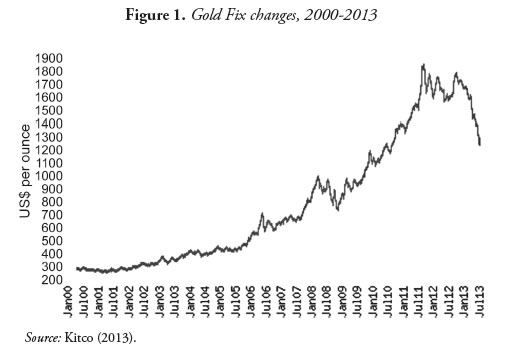
Looking at the historical nominal prices (i.e., the fix), there was for the year 1990 a 'climb' to $383.52 USD/Oz and in the late nineties a fall to $270.91 USD/Oz. This rose up again precisely in 2002, and in 2011 rose to the startling figure of $1,875 USD/Oz, which became a ceiling for the price of gold. This fragile bubble bursts in September of 2011, and the price dropped about $300 USD/Oz. Since then, it seems to have stagnated between $1,600 USD/Oz and $1,800 USD/Oz, to fall lately to prices in the order of $1,200 up to $1,300 USD/Oz since April 2013, caused by the U.S. slight recovery, which transmitted more confidence to investors in the stock market and sectors of productive industry other than gold mining (see Figure 1).
But how does one explain these changes? What generates so much volatility in gold prices? What will be the upper and lower limits? What will be the pace of its rise or fall in the coming years? Arriving at these answers is not simple but through economic analysis taking into account the historical, cyclical movements of gold price in relation to stock markets, it becomes possible to approximate to reality. Such cyclical movements are a dominant feature of commodity prices (Cashin, McDermott & Scott, 2002), an observation that guides this research to its conclusions.
In this paper, the phenomenon of changes experienced by gold prices is handled in the context of a 37–year history–that is, one complete period as explained below.
Analysts have attempted to forecast gold price behavior by using several methodologies, like Markov chain combination model, BP neural network model and Grey Markoff model for the Chinese case of study. Also, the Factor augmented VAR model (Lili & Chengmei, 2013) was used to model the nominal prices of the metal over time, which the authors admit is very rough to even predict gold prices with the required accuracy the decision makers need. And it is a natural thing, for gold prices are very volatile, and therefore hard to predict, thus making gold mining itself a very high risk activity in financial and economic terms (Shafiee & Topal, 2010). Based on the latter statement, the idea of using linear or nonlinear regressions, as well as autoregressive models like ARMA, ARIMA, GARCH, among others, is discarded, because the volatility of gold prices make them all rough approximations to reality, only useful to predict in the short term. Modeling gold prices in relation to its determinants is a good proposal, like the relation between gold and platinum prices to their offer and demand in the market (Kearney & Lombra, 2009) and the macroeconomic determinants of gold prices (Batten, Ciner & Lucey, 2010). Another good model for predicting gold prices could be made by using neural networks (Parisi, Parisi & Díaz, 2008), which is fed by a lot of data, it is, daily prices of the metal constantly updated; but the predictions it can yield are of an acceptable accuracy some days ahead of today (even less than a week), and it does not work for making long-term predictions for the real dynamics of changes in prices have to be known and fed to the model in order to predict only the short-term outcomes. This is not useful for decision makers, who need to know with a great deal of accuracy the price of gold in the far future, which is still such a hazardous task to be done due to the volatility of gold prices.
B. The Dow Gold ratio
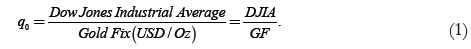
A good model to be proposed in light of the described problems of gold prices themselves is the analysis of the ratio of the Dow Jones stock market index (i.e. the Dow Jones Industrial Average, defined as the value of the shares of the 30 largest companies listed on the NYSE) and the price of gold in USD/Oz, or the DJIA/GF ratio variable (Prechter, 2009), by means of which Robert Prechter found that an economic recession was taking place since year 2000. For it was always decreasing, like it did during the 1930s and 1970s world economic crises, Prechter identified a cyclical behavior in this ratio variable but did not prove it with mathematical arguments, which is done in this paper. This ratio is shown in Equation (1):
The problem of volatility and the rapid change with which gold prices have to be predicted is eliminated with the DJIA/GF ratio, which changes slowly throughout the years and whose relation to the booms and busts of the world economy is evident, if one is a good observer.
C. Booms and busts of the world economy in light of the DJIA/GF
The trajectory of this Dow Gold ratio throughout the twentieth century traces two complete cycles, and almost half of a third currently underway. When the DJIA/GF ratio increases (i.e. the curve rises), it is because investors prefer to turn their investments to the stock market, leaving gold in second place. This is seen after World War I until the 1929 crisis, and also in the fifties, most of the sixties, and the nineties. These were times of prosperity forged by the expectation of unlimited industrial production and growth, which led a huge mass of speculators to buy shares in companies considered safe and profitable. A decreasing DJIA/GF ratio has been reflected in the crisis of 1929, when stock prices stopped rising and the DJIA/GF ratio went into a free-fall lowering, which tells about an increasing investors' preference for gold (whose price rose in the same period). The same happened in the late sixties and the seventies continuing up to the speculative mirage of 1980. The market has been experiencing a period of rising gold prices, along with the stagnation of stock prices throughout the period 2000-2013 (see Figure 2), and the decreasing DJIA/GF is a good indicator of this.
The turning point of the trend of the DJIA/GF ratio is the shift from one market to another and the last point of the base of the curve is that ''magic roof '' that reverses the expectations. The opposite occurs at the peak of the curve: for instance, a growing financial imbalance that predicts high ceilings like $1,000 USD/Oz in 2006, $1,875 USD/Oz in 2011, and a slight economic recovery that is reflected in a fall to $1,200 USD/Oz in 2013. In the 1930s, a short downward trend in the stock market took place between 1929 and 1933. The recovery of the U.S. economy represented by the growth of the Dow Gold ratio did not stabilize until 1942 or so; therefore, the period from 1929 to 1942 is considered a descending half-cycle. The second descending half-cycle, from 1966 to 1980, lasted 14 years. The third descending half cycle meant a long period favorable for gold beginning in 1999, which could be projected until the middle or even latter part of the 2011-2020 decade. An average half-cycle has been found to last 18.5 years, with the complete cycle lasting 37 years. The period represents the distance in time between two consecutive local minima or maxima, as explained later by using Fourier analysis. However, the current half-cycle is different from the previous two due to significant influencing factors this time around. The global financial system, in its current form, is unimaginably large with ever-growing volumes of capital, large debts like those held by the United States treasury, virtual capital ''derivatives'', deficits created by expansionary monetary policies, among others. These factors grow the bubble, allowing gold prices to reach new heights.
D. Influential Factors on Gold Prices
Three groups of influential factors are described to affect gold prices (Lili & Chengmei, 2013):
a. Financial market: This one has a converse influence: when gold goes up, financial indicators decline and vice versa. Gold competes with the currency, financial options of investment; and global investors assess one of them, gold or the financial markets, the one that is more profitable to invest in.
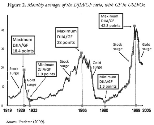
b. Gold reserves and energy prices: As the main purchasers of gold, central banks hold most of the gold that is present in the global market. The idea that central bankers have already sold much of their gold and that future sales will be further restricted has spread worldwide, but it depends on gold prices, which have to be high for it to happen. As oil price rises, it is accompanied by an increase in the price of gold. Their prices are correlated because both belong to the category of commodities. Although the global economic recession of 2008 reduced oil prices temporarily, they have maintained an upward trajectory during the period 2000-2013 (see Figure 3).
c. Macroeconomic factors: Variables like CPI, inflation, interest rates, government bond prices, among others, influence gold prices conversely. For instance, political tensions, social and religious conflicts, etc., generate international political instability, and in turn lead growing numbers of investors to direct their gaze toward gold to hedge or replace riskier investments, for they increase inflation and interest rates, take low stock prices, making the gold more attractive. The opposite is true: when society is in a good level of order, business in stock markets is more attractive than investing in gold, which will have lower prices then.
II. Conceptual Framework
A. Fourier analysis
1. Fourier series modeling
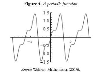
The Fourier series is aimed to decompose a periodic function into the sum of pure oscillating signals, namely sines, cosines, or complex exponentials. This decomposition of periodic functions is a part of the very Fourier analysis. Each of the terms of the series in which the function is decomposed is called a harmonic, and every harmonic has a frequency that is always n times the fundamental frequency (the frequency of the first harmonic), where n is an integer.
A periodic function F(t) is such that it couples with the form presented in Equation (2):

where p is the period of the function. The graph of F(t) can be made by repeating the very graph within any interval of length p. A periodic function is such that a given interval of length p, where p is the period, repeats its graph over and over again throughout the time line. An example of a periodic function can be seen in Figure 4.
The Fourier series of a periodic function F(t) (Kreizig, 2006) is given by Equation (3):

where F(t) is the Fourier representation of the DJIA/GF ratio as a function of time t, an is the magnitude coefficient of the nth harmonic, n is the number of the harmonic, i.e. an integer larger than zero, ωf is the fundamental frequency or the one corresponding to the first harmonic, t is a year from, and θn is the phase angle of the nth harmonic.
In fact, a harmonic is a pure periodic cosine wave of the form shown in Equation (4):
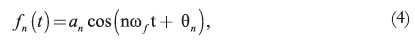
where fn(t) n f t is the n-th harmonic of the Fourier series. The period of the n-th harmonic can be found in Equation (5):
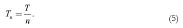
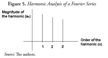
2. Fourier harmonic analysis
One way in which a frequency sweeping, so to speak, could be done over a periodic function is to plot on the horizontal axis the order of every harmonic, and on the vertical axis the magnitude of every harmonic, in order to compare their magnitudes and analyze which of them affect more the series, or in fact domain it −as some times happen, when the magnitude of some harmonics are evidently higher than the rest. The magnitudes of each of the harmonic terms of a periodic function that form a Fourier series are plotted one by one, with the horizontal axis representing the order of the harmonic (n) and the vertical one its magnitude (an). The former is called a harmonic analysis (see Figure 5).
B. Neural Networks as Predictive Models
1.The prediction
Neural networks is widely used for different kinds of applications (Straßburg, Gonzàlez-Martel & Alexandrov, 2012; Timo, Klapuri, Saarinen & Ojala, 1996; Yonaba, Anctil & Fortin, 2010). One of the main problems of Neural Networks (NN) is that there is not a consensus as to how to best use them (Yonaba et al., 2010). And because of this fact, several simulations and adjustments to a NN model have to be done before considering it a one that fits the data, and thus to be considered a good estimator.
Neural networks can be used to model time series, having the advantage of fitting the data better than other models like ARMA, ARIMA, GARCH, etc., because the back propagation error is minimized dynamically as the model learns how the time series behaves, and reduces the error to the closest to zero value possible for every run.
Neurons form the basic unit of a NN (Yonaba et al., 2010). The input data feeding the model is a vector of data, the time series real data, that is, x =(x1, x2 , x3 , x4 ... xt ) where t is the number of neurons used for acquiring one prediction  at the time t. The parameters are stored in the arrays w=(w1, w 2 , w 3 , w 4 ... w t for the weights, and b=(b1, b 2 , b 3 , b 4 ... b t)for the biases. The total synaptic input, uk , is then found using Equation (6):

where k is the number of the hidden layer to be used.
Now the estimated is found by means of Equation (7), and it is the prediction that the model yields for the time N:

where Θ1 and Θ2 are transfer functions, i and k represent indexes, K is the number of hidden layers implemented (K = 2 for the case of study), and t represents the number of lags used to predict , xt that is, the number of neurons of each layer (10 for the case of study). The linear transfer function is shown in Equation (8), and it is used in the outer layer for the case of study:
Other common transfer function is the logistic sigmoid, shown in Equation (9), and it is used for the hidden layer in the case of study:

2. Performance of the model: quality of the prediction
The predictive model is proved predicting known data, then comparing the estimation xt with the real value. xt The objective function is the Mean Square Error, MSE, which is to be minimized in order to have the best performance of the NN model. The process is also called Training of the NN. The RMSE is found by means of Equation (10):

where n is the number of observations.
A restriction that guarantees a non-biased prediction is to have the absolute errors totalizing zero, as shown in Equation (11):

To measure the performance of an NN model, the Nash and Sutcliffe efficiency index (1970) is suggested (Yonaba et al., 2010). The CR1 is tailored as a coefficient of variation, but it ranges from  to 1. It approximates 1 for an almost perfect fit between the NN model and the data. To find it, use Equation (12):
where is the average of the x =(x1, x2 , x3 , x4 ... xt ) set.
III. Analysis of the DJIA/GF ratio
A. Fourier analysis for the DJIA/GF Time Series
Analysis of the ratio of the Dow Jones Industrial Average and Gold Fix makes it possible to model the cyclicality of gold prices themselves. This analysis uses a Fourier series model suitable for cyclical variables, and analyzes annual closure data from 1900 to 2010. This was implemented by developing an application that works under the MATLAB software. Clearly, this way of modeling the DJIA/GF is discarded to be used as a predictive model, for the series is taken as periodic throughout 1900-2010, which is not the real case, because the DJIA/GF does not fulfill the strict definition of a periodic function. The purpose of this analysis then is to decompose the series of the DJIA/GF into its harmonic components, to compare their magnitudes, and to explain through them why the troughs and peaks of the series have an almost constant separation in time, i.e., approximately 37 years. If the number of harmonics is high enough to minimize the error between the real data and the Fourier series model, then that model is acceptable. When a finite number of harmonics is used, then Equation 13 would be the finite Fourier series of the data:

where N is the number of harmonics used for adjustment of the DJIA/GF series.
The mean error estimation is found by means of Equation 14:
To minimize this error, and its corresponding minimum mean error, the optimal number of harmonics for the adjustment of the DJIA(t)/GF (t) time series within the MATLAB simulation is found to be N =55, E = 1.55 * 10-14.
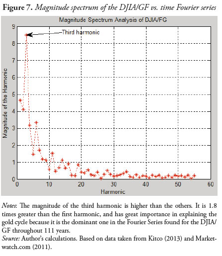
By means of a magnitude spectrum analysis on the named Fourier series, which consists of a graphic of the harmonic n vs. its magnitude , an, we find the third harmonic magnitude to be considerably larger than the others: i.e. 1.8 times greater than the first harmonic, which is the second in magnitude, and 2.5 times greater than the sixth, which is third in magnitude. This can be seen in Figure 7. On the other hand, Figure 6 illustrates an even more interesting finding: the third harmonic has its highest and lowest points very close in time to the corresponding high and low points of the DJIA/GF ratio time series.
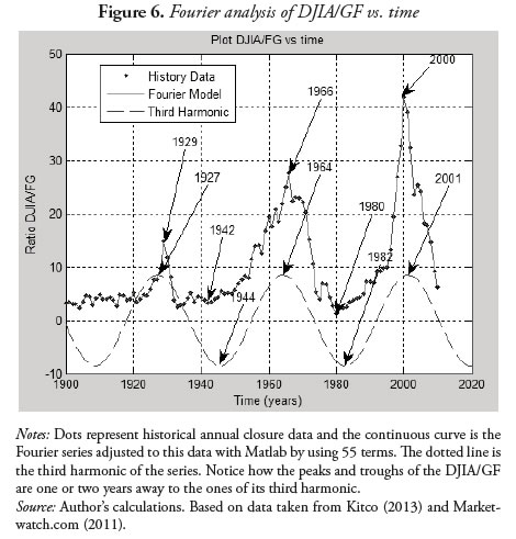
The third harmonic of the Fourier series (n = 3) is described by Equation (15) and can be seen in Figure 6:

To find the fundamental frequency, Equations (16) and (17) are the right tool:
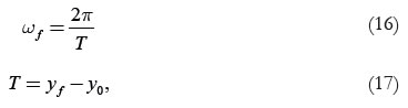
where T is the time span analyzed, yf y is the final year of the time span analyzed, and y0 is the initial year of the time span analyzed.
The fundamental frequency ωf is calculated from data available from T = 111 years, namely:
where T3 is the period of the third harmonic.
We are therefore faced with the important observation that the DJIA/GF ratio does behave cyclically, and that a pure wave with a period of 37 years (i.e. the time between two peaks or two valleys) helps to understand what happened in 1929, for example, when there was a relative maximum that then became the starting point for a succession of falls until 1933, when it reached a relative minimum. Throughout the ongoing decade, its values remained below 5, showing a tendency to stagnate. It experienced another relative minimum in 1942; and it was not until 1946 when it managed to exceed the value of five, 17 years after 1929, where it held for 3 years barely above 5, and showed a determined upward trend from 1949 onward (the beginning of the 50s boom).
Now let's observe the behavior of the DJIA/GF ratio. The minimums in 1946 and 1980 are separated by 34 years, maximums in 1929 and 1966 separated by 37 years, and maximums in 1966 and 2000 separated by 34 years. It is now clear why this third harmonic is greater in magnitude than the rest of the 55 calculated in the named Fourier series, and therefore it is the most important. These findings are reinforced by the fact that over the period of 111 years, this behavior is observed to be cyclical, and it seems to continue behaving the same way. Despite a fall in gold prices during April 2013 and after that, and they continued to show a tendency to stagnate in yet high market values, while the stock market remained in a state of stagnation or slight recovery at best. This is reflected in a DJIA/GF ratio that seems to be tending to fall below five again after 2010 (see Figure 6). Accordingly, in about the year 2020, this ratio should experience a new surge, (i.e. a rebound in stocks) with the result that gold prices will fall back to lower ''normal'' values with a tendency toward stagnation. This is not certain since this point may occur up to 2 years before or after 2020 or so, based on previous observations, but from this point it is clear that, at most, by the end of the 2011-2020 decade, the gold rush will begin to vanish.
B. Analysis of the Ratio DJIA/GF by Means of Neural Networks
1.Predictive model
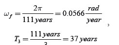
To make a specific predictive model, we have used the Neural Networks algorithm, which in this case, has 1 input layer of data, 2 hidden layers (K = 2), and the respective output xt (i.e. the sought prediction, see Figure 8). The question to be answered here is: how many data must be used to train the network, so as to obtain the best prediction possible? Since the interest is in making a valid prediction for the 2011-2020 decade, models using 3 to 10 neurons were tested (i.e. both the input layer and two hidden ones were trained with data from three to ten years before the year in which the prediction was sought). The model that resulted in the lowest mean squared error was the one using 10 neurons, as reported in Table 1. The Microsoft Excel Solver application was used to calculate the weights wi in each of the model tests to minimize the mean squared error in each case, so as to achieve a superior predictive model.
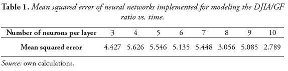
In the case of the 10 neurons model, the mean squared error is 2.789, less than the others. It follows that its mean absolute error is 1.670, meaning that on average each point in the time series of the DJIA/GF ratio is that far from each point of the predictive model; and the Nash and Sutcliffe efficiency index CR1 = 0.977 is very close to 1, which indicates a good fit between the model and the real data. Furthermore, a restriction was imposed in all of the cases on the total relative error so that each of the relative errors between the predictive model and the actual data fit an unbiased normal distribution, thus ensuring the reliability of the resulting predictive model. The plot of this model and the real time series can be seen in Figure 9.

3. Reliability of the prediction
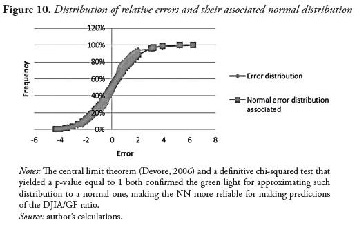
The distribution of errors in this case fits a normal distribution following the Central Limit Theorem CLT (Devore, 2006), as can be seen in Figure 10. A definitive chi-squared test confirmed that the error distribution fits normal parameters (the yielded p-value was 100%), and therefore the variance can be taken as a constant. Hence, a confidence interval of 95% can be established for the DJIA/GF ratio, which takes as its centerpiece the prediction obtained from the neural networks model and ranges about two standard deviations above and below the center. Mathematically, this is written as in Equation (18):

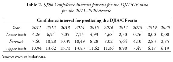
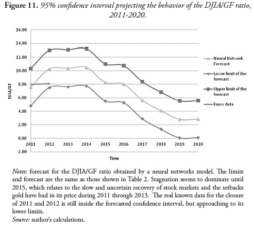
Where  (t) is the value of the DJIA/GF ratio estimated or predicted by the neural network model; σ is the standard deviation of the named model with respect to the actual data; q(t) is the actual value of the DJIA/GF, and 95% is the probability of the real closing value of the ratio to remain inside the confidence interval. From the proposed model above, Table 2 and Figure 11 were constructed.
IV. Discussion of Results
A. What the mathematical models tell
It is clear that the DJIA/GF is a cyclical ratio of help to understand the gold cycle by allowing analysts to go beyond the figure of the nominal price, which is more volatile and therefore uncertain. Almost every 37 years the circumstances repeat about the gold market, it has been like that during the 20th century and throughout the first years of the 21st, and it is expected to have things behaving the same way for an undefined time. The Fourier analysis tells us about cycles, and neural networks about the most probable events to happen in the near future, and both reach a common conclusion: at most 2 years before 2020, the DJIA/GF will have a sustained recovery to give birth to a new cycle.
What has happened throughout the period 2011-2013 reflects what the NN model predicts: a stagnation of the DJIA/GF ratio. This stagnation is related to gold price stagnation and low, day-to-day increases in the DJIA: changes which barely compensate for the falls it experiences some days. Up to the present moment, this model is assertive in its confidence interval when compared to real data: it is not just the numbers that tell analysts what is going to happen, but the historic gold cycle itself.
B. What the political circumstances tell
While there is uncertainty about the effects of spending cut policies implemented by the U.S. government (Alvarez & Rodríguez, 2011), it is probable that they should eventually bring back confidence in the economy of that country; so the trend of the Dow Jones Industrial Average would be upward, accompanied by a decline in gold prices, as happened in 2013. However, the troubled negotiations over the decision to increase the debt ceiling have played a negative role and diminished confidence. It is very interesting to see how the 10-node neural network model gives a positive prediction for the years 2012 to 2015 as far as the stock market is concerned for this reflects the way a reasonable person would think of the market when analyzing historiGutiérrez, Franco y Campuzano: Gold prices: Analyzing its cyclical behavior cal trends. Recall that in the 1930's and 1970's (1937 and 1976, specifically), times of global economic recession, the ratio climbed up temporarily, then fell again to the bottom, and then increased steadily over a period of about 18.5 years.
Conclusions
Gold prices are very volatile to be predicted with accuracy in the long term; however, they behave cyclically in relation to stock market indexes, as was seen in the case of the Dow Gold ratio or DJIA/GF. This knowledge opens a door for better understanding the behavior of gold prices in the long term. Gold prices are affected by three things: financial markets, energy prices and reserves, and macroeconomic indicators. As gold is a commodity, it tends to behave in a positive relation to energy prices and in a negative relation with financial markets and macroeconomic indicators. It is so, because gold is seen as a safe haven when hazardous times hit the global economy, and taken to a second place when the economy is doing well and thus it is more attractive to invest in companies than in gold itself.
Although the supply of gold on the international markets is negligibly increased by small gains in production and some central banking policies, these increases are not enough to meet the demand that has been going on since the financial crisis of 2008, resulting in a gold deficit for covering a stock market and macroeconomic downfall that may occur. In other words, the supply of gold, although increasing slightly in absolute terms, is generally decreasing in terms of availability in this kind of circumstances. The gold rush then is predicted to be stronger after 2015, and a repetition of history would take place if that happens, that is, gold prices would increase dramatically as the Dow Gold ratio tends to fall again.
If policies to counteract the economic slowdown in this decade imposed by the United States and other nations yield positive results, it is expected that the DJIA/GF ratio will behave positively as predicted by the Neural Networks model proposed in this paper. Specifically, the DJIA/GF ratio will closely correspond to the upper limit of the proposed confidence interval,
or with less probability, surpass it. Market watchers must be vigilant while following this trend in 2013, which in turn is behaving the opposite way. In order to anticipate what will happen until about 2020 or before, it is crucial to know what will happen in the short term, especially if the monetary policies implemented worldwide should fail in their purpose.
The periodicity of the Dow Gold ratio of 37 years indicates that with this figure, it is possible to find similar circumstances to today's about the gold market itself; for instance, the 1970s crisis was taking place 37 years ago, and the 1929s crisis took place 74 years ago, having as a direct consequence high gold prices and low stock market values for shares of most companies. Slight recoveries take place after measurements are made by governments in an effort to save the economy, they work temporarily, another crash comes, and finally a steady recovery shows up. The converse situation happens too; that is, 1950 and 1987 are 37 years away, and in these years an economic recovery after a crisis was taking place in the world economy, making gold prices go down while stock prices and macroeconomic indicators were going in a steady uptrend.
REFERENCES
Aizenman, Joshua & Inoue, Kenta (2013). ''Central banks and gold puzzles'', Journal of the Japanese and International Economies, Vol. 28, pp. 69–90. [ Links ]
Álvarez, Jose & Rodríguez, Eduardo (2011). ''Long-term Recurrence Patterns in Late 2000 Economic Crisis: Evidences from Entropy Analysis of the Dow Jones Index'', Technological Forecasting and Social Change, Vol. 78, Issue 8, pp. 1332–1344. [ Links ]
Batten, Jonathan; Ciner, Cetin & Lucey, Brian M. (2010). ''The macroeconomic determinants of volatility in precious metals markets'', Resources Policy, Vol 35, Issue 2, pp. 65–71. [ Links ]
Baur, Dirk G. & Mcdermott, Thomas K. (2010). ''Is gold a safe haven? International evidence'', Journal of Banking and Finance, Vol. 34, Issue 8, pp. 1886–1898. [ Links ]
Cashin, Paul; McDermott, John C. & Scott, Alasdair. (2002). ''Booms and Slumps in World Commodity Prices'', Journal of Development Economics, Vol. 69, Issue 1, pp. 277–296. Retrieved from http://www.sciencedirect. com/science/article/pii/S0304387802000627 (April 27,2013 ). [ Links ]
Christie–David, Rohan; Chaudhry, Mukesh & Koch, Timothy W. (2000). ''Do macroeconomics news releases affect gold and silver prices?'', Journal of Economics and Business, Vol. 52, Issue 5, pp. 405–421. [ Links ]
Craig, Lee A.; Fisher, Douglas & Spencer, Theresa A. (1995). ''Inflation and money growth under the international gold standard, 1850–1913'', Journal of Macroeconomics, Vol 17, Issue 2, pp. 207–226. [ Links ]
Devore, Jay L. (2006). Probabilidad y Estadística para Ingeniería y Ciencias. California, San Luis Obispo: International Thomson editores. [ Links ]
Kearney, Adrienne A. & Lombra, Raymont E. (2009). ''Gold and platinum: Toward solving the price puzzle'', The Quarterly Review of Economics and Finance, Vol. 49, Issue 3, pp. 884–892. [ Links ]
Kitco (2013). 10 Year Gold. Retrieved from: http://www.kitco.com/charts/popup/au3650nyb.html (March 03, 2013). [ Links ]
Kreizig, Erwin (2006). Advanced Engineering Mathematics (9th ed). Hoboken, NJ: Wiley Eastern.John Wiley & Sons, Inc. [ Links ]
LBMA (2012). London Bullion Market Association. Retrieved from http://www.lbma.org.uk/pages/index.cfm (March 15, 2013). [ Links ]
Lili, Li & Chengmei, Diao (2013). ''Research of the Influence of Macro- Economic Factors on the Price of Gold'', Procedia Computer Science, Vol. 17, pp. 737–743. [ Links ]
Lothian, James R. (2002). ''The internationalization of money and finance and the globalization of financial markets'', Journal of International Money and Finance, Vol. 21, Issue 6, pp. 699–724. [ Links ]
Marketwatch.com (2011). Dow Jones Industrial Average. Retrieved from http://www.marketwatch.com/investing/index/djia (December 21, 2011). [ Links ]
Mollick, Aandrè Varella & Assefa, Tibebe Assefa (2013). ''U.S. stock returns and oil prices: The tale from daily data and the 2008–2009 financial crisis'', Energy Economics, Vol. 36, pp. 1–18. [ Links ]
Neuro Dimension Inc. (2012). Neuro Dimension. Retrieved from: http://www.nd.com/neurosolutions/products/ns/whatisNN.html (September 21, 2012). [ Links ]
Parisi, Antonino; Parisi, Franco & Díaz, David (2008). ''Forecasting gold price changes: Rolling and recursive neural network models'', Journal of Multinational Financial Management, Vol. 18, Issue 5, pp. 477–487. [ Links ]
Prechter, Robert (2009). Gold & Silver. Retrived from: http://www.bullionworks.com/images/Gold_Silver_Ebook.pdf (March 03, 2013) [ Links ]
Shachmurove, Yochanan (2011). ''A historical overview of financial crises in the United States'', Global Finance Journal, Vol. 22, Issue 3, pp. 217–231. [ Links ]
Shafiee, Shahriar & Topal, Erkan (2010). ''An overview of global gold market and gold price forecasting'', Resources Policy, Vol. 35, Issue 3, pp. 178–189. [ Links ]
Smith, Eric & Shubik, Martin (2011). ''Endogenizing the provision of money: Costs of commodity and fiat monies in relation to the value of trade'', Journal of Mathematical Economics, Vol. 47, Issue 4-5, pp. 508–530. [ Links ]
Straßburg, Janko; González-Martel, Christian & Alexandrov, Vassil (2012). ''Parallel genetic algorithms for stock market trading rules'', Procedia Computer Science, Vol. 9, pp. 1306–1313. [ Links ]
Timo, Hämäläinen; Klapuri, Harri; Saarinen, Jukka; Ojala, Pekka & kaski, Kimmo (1996). ''Accelerating genetic algorithm computation in tree shaped parallel computer'', Journal of Systems Architecture, Vol. 42, Issue 1, pp. 19–36. [ Links ]
Williams, James L. (2012). Oil Prices History and Analysis. Retrieved from: http://www.wtrg.com/prices.htm (September 21, 2012). [ Links ]
Wolfram Mathematica (2013). Fourier Series. Retrieved from: http://reference.wolfram.com/legacy/v8/ref/Files/FourierSeries.en/O_2.gif (July 17, 2013). [ Links ]
Yonaba, H.; Anctil, F. & Fortin, V. (2010). ''Comparing Sigmoid Transfer Functions for Neural Network'', Journal of Hydrologic Engineering, Vol. 15, Issue 4, pp. 275–283. [ Links ]
