


 English (pdf)
 Article in xml format
 Article references
 Send this article by e-mail
 Cited by SciELO
  Cited by Google
  Similars in
SciELO
Similars in
SciELO  Similars in Google
 Permalink
Introduction
Traditionally, no arbitrage affine term structure models (ATSMs) assume that the yield curve is jointly spanned by all state variables. Empirical evidence originally suggests that the yield curve is sufficiently described by three latent yield factors, which are often called "level", "slope" and "curvature" (see Litterman & Sheinkman, 1991; Ang and Piazzesi, 2003; Diebold & Li, 2006). More recently, Cochrane and Piazzesi (2005), Cochrane and Piazzesi (2014) and Duffee (2011) highlight the importance of additional factors; and Adrian, Moench and Crump (2013) show that the first five principal components of Treasury yields are needed in order to explain Treasury returns. However,
the yield curve does not contain all available information to forecast future excess bond returns. In fact, Ludvigson and Ng (2009) argue that: "real and inflation factors have important forecasting power for future excess returns on U.S. government bonds, however this behavior is ruled out by the affine term structure models where the forecastability of bond returns and bond yields is completely summarized by the cross-section of yields or forward rates." Lastly, Joslin, Priebsch and Singleton (2014) find that the additional information in macroeconomic variables that predicts excess bond returns is not perfectly spanned by the yield curve.
While macroeconomic variables such as real output and inflation have usually been proposed as unspanned factors, little attention has been paid to financial market variables as possible additional unspanned factors.2 This paper examines the role of liquidity risk premium as an unspanned factor for the U.S. term structure. In particular, the aim is to determine whether or not liquidity risk has an impact on bond investment decisions apart from the effect of the traditional bond yield factors. This is motivated by recent empirical findings suggesting that bond excess returns can be predicted by liquidity risk, and therefore could be considered as an unspanned factor that forecasts bond returns but is not necessarily spanned by the yield curve.
A variable is unspanned if its value is not related to the contemporaneous cross section of interest rates, but it helps to forecast future excess returns on bonds (i.e., term structure risk premia). There are numerous studies that identify financial and macroeconomic variables as predictors for the U.S. bond risk premia (expected excess returns). For instance, the term structure slope, the forward spread, the lagged excess returns, the Cochrane and Piazzesi's (2005) tent-shaped factor, and macroeconomic fundamentals are some of the variables that have been identified as predictors for Treasury bonds (see Fama, Euegen & Bliss, 1987; Campbell, Shiller & Viceira, 1991; 14 Cochrane & Piazzesi, 2005; Ludvigson & Ng, 2009; Cooper & Priestley, 2009). Also, the role of liquidity as a predictor variable has been studied by Fontaine and Garcia (2012), Pflueger and Viceira (2012) and Gomez (2015). These studies provide empirical evidence for liquidity as a source of predictability for U.S. Treasury bonds, Treasury Inflation-Protected bonds (TIPS), or for both.
Unspanned factors in macro-finance term structure models are a topic of recent interest. The identification of unspanned risk is important as traditional spanned factors that capture the cross section of interest rates are not able to completely explain the physical dynamics of the data. Yet the literature has concentrated its search on spanned variables embedded in the U.S. term structure. As result, a set of candidates besides the traditional bond yield factors have been identified, among which macroeconomic fundamentals are the most popular (see Cochrane & Piazzesi, 2005; Hordahl & Tristani, 2010; Cochrane & Piazzesi, 2014; Kim, 2009; Cooper & Priestley, 2009; Ludvigson & Ng, 2009; Orphanides & Wei, 2010; Chernov & Mueller, 2012, among others). Based on this evidence, macro-finance models have been proposed by Ang and Piazzesi (2003), Moench (2008), Diebold, Rudebusch and Aruoba (2006), Lyrio and Maes (2006), Dewachter and Lyrio (2006), Rudebusch and Wu (2008), Bekaert, Cho and Moreno (2010), and Dewachter and Iania (2011). However, the assumption underlying these models is that macroeconomic fundamentals are fully spanned by the term structure, an assumption that is not empirically supported.
In response to this, Duffee (2011), Boos (2011) and Joslin et al. (2014) introduce a new branch of ATSMs where state variables have an effect on bond risk premia but do not span the cross-sectional distribution of yields. In particular, Duffee (2011) introduces unspanned hidden factors and documents that these are an economically important component of bond risk premia. Boos (2011) extends a term structure model of the Ang and Piazzesi (2003) class with unspanned macro factors, and provides an example with survey data on expected inflation to filter an unspanned factor. Lastly, Joslin et al. (2014) explicitly apply unspanned factors to observed macroeconomic variables (i.e., the inflation rate and industrial production growth), and show that shocks to those variables have a significant effect on the U.S. term premia.
In this paper, I formally test for the unspanning properties of liquidity risk in the context of a joint Gaussian ATSM for zero-coupon U.S. Treasury and TIPS bonds. The liquidity factor is restricted to affect the cross section of yields, but it is allowed to determine bond risk premia as well. In other words, I consider liquidity as an additional factor that does not span the yield curve, but improves the estimation of bond risk premia. Using this empirical model, I attempt to answer the following questions: (i) Is it plausible to consider the liquidity premium as a factor that forecasts bond returns, but which is not spanned by the yield curve? (ii) Does the liquidity factor affect the dynamics of bonds under the pricing measure, but does affect them under the historical measure? And if so, how does the market price liquidity risk in the U.S. government bond market? (iii) Does the variation in the liquidity premium influence the yield curve factors? An affirmative answer to these questions will define a factor as unspanned by the yield curve.
Theoretically, less liquid securities carry higher liquidity risk, and thus must carry a higher yield (i.e., higher expected returns or risk premia as well) as a compensation for the incremental risk and the higher cost of trading. This additional yield is the liquidity risk premium. A comparison of TIPS' lack of liquidity with nominal Treasuries results in TIPS yields having a liquidity premium relative to Treasuries. In fact, the liquidity differential of TIPS relative to Treasury bonds has been well documented in the literature (see Sack & Elsasser, 2004; Shen, 2006; Hordahl & Tristani, 2006; Campbell, Shiller & Viceira, 2009; Dudley, Roush & Steinberg, 2009; Christensen & Gillian, 2011; Gurkaynak, Sack & Wright, 2010; Pflueger & Viceira, 2012).
I identify the liquidity component in TIPS yields through the difference between the observed break-even inflation rates (BEI) and the inflation swap rates, the latter regarded as synthetic BEI. This measure was first introduced by Christensen and Gillian (2011) and combines information from the U.S. bond market with information from the inflation-indexed swaps market, which is recognized as the market that trades the most liquid inflation derivatives in the over-the-counter (OTC) market. The particular choice of this measure for the liquidity premium is motivated by three facts: First, it is highly correlated with other measures of the TIPS liquidity premium available in the literature, suggesting that they are all capturing similar information about the liquidity differential between nominal and TIPS yields. Second, U.S. bond excess returns can be predicted by this liquidity measure. Third, it is a market-based measure of liquidity that is straightforward to compute.
I start by empirically testing the plausibility of the TIPS liquidity premium as an unspanned factor. I find that the TIPS liquidity premium fulfill the three empirical facts identified by Joslin et al. (2014) in the case of macroeconomic variables. First, the TIPS relative liquidity premium is not linearly spanned by the information in the joint yield curve. Second, the unspanned liquidity factor has predictive power for excess returns in bond markets. And third, bond yields follow a low-dimensional factor model.
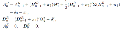
Next, I estimate the joint pricing model of TIPS and Treasury bonds by using the three-step linear regression procedure introduced by Adrian et al. (2013), and adapted by Abrahams, Adrian, Crump and Moench (2015) in the case of joint bond pricing. This procedure has the advantage of being easily implementable and computationally efficient; also, it allows a large number of pricing factors and can accommodate unspanned factors. From the estimation of a five-factor model (including four principal components of zerocoupon yields, plus the liquidity premium as pricing factors), I test for the presence of unspanned factors. I present empirical evidence suggesting that the liquidity factor does not affect the dynamics of bonds under the pricing measure, but does affect them under the historical measure. Consequently, the information contained in the yield curve appears to be insufficient to completely characterize the variation in the price of curvature risk.
Finally, to confirm if liquidity factors are truly unspanned by the yield curve, I test whether liquidity has predictive information for the yield curve factors. To do that, I examine the empirical relationship between movements in the level, slope and curvature of the term structure of U.S. nominal and real interest rates and TIPS liquidity premium shocks. As is traditional in this empirical literature, I infer the relationship between yield movements and shocks to liquidity using impulse-response functions (IRFs) implied from a vector auto-regression model (VAR). Results show that the TIPS liquidity premium influences the shape of the joint nominal and real yield curve. More so, shocks to nominal and real bond yield factors appear to have an effect on the liquidity premium. This effect is meaningful given that, as previous empirical evidence has shown, yield curve factors are highly correlated with measures of inflation expectations and monetary policy instruments, which provides an explanation for this dynamic connection.
The rest of the paper is organized as follows. Section I describes the joint term structure model for nominal Treasury and Inflation-Linked Bonds (ILBs), and the estimation procedure. I describe the data and the set of pricing factors in Section II. Section III presents the main empirical findings. The last section concludes.
I. Affine Gaussian term structure model with unspanned risk
In this section, I introduce the ordinary Gaussian ATSM framework proposed in discrete time by Abrahams et al. (2015) for pricing ILBs jointly with nominal bonds, so that both yield curves are affine in the state variables. However, in the spirit of Joslin et al. (2014), in addition to the yield curve risk (principal component factors), I consider liquidity as a different source of risk in this model, which is unspanned by the joint yield curve.
A. Setup
Consider a discrete time environment. Let  denote the price in dollars at time t of a nominal zero-coupon bond that pays out one dollar at the maturity date n. Let It
be any stochastic process at time t. I denote by
denote the price in dollars at time t of a nominal zero-coupon bond that pays out one dollar at the maturity date n. Let It
be any stochastic process at time t. I denote by  the price in dollars at time t of a contract that pays out It dollars at time n. If It denotes the consumer price index (CPI) at time n, then it is the price at time t of a contract that pays out the dollar value of one CPI-unit at maturity. Hence, in this case, Pt,nR is the price of an inflation-linked zero-coupon bond, which I will refer to as a real bond hereafter.
Assume that a liquid riskless nominal zero-coupon bond price at time t with maturity n is given by
 , ()1
, ()1
where denotes the expected value at time t under the risk neutral measure Q, and rt
N
is the nominal risk-free interest rate. Similarly, the price at time t of an inflation-linked zero-coupon bond that matures at time n is equal to
denotes the expected value at time t under the risk neutral measure Q, and rt
N
is the nominal risk-free interest rate. Similarly, the price at time t of an inflation-linked zero-coupon bond that matures at time n is equal to
 ()2
()2
where
r
t
R
is the real interest rate. In this case, ILBs are priced by discounting future cash flows using a real short rate. Note that this short rate is equal to the difference between the nominal one and the inflation rate, .
.
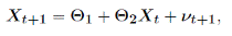
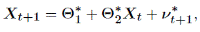
Working in a general affine framework, I assume that the dynamics of the
K ×1 vector of state variables Xt under the historical measure P is given by
 ()3
()3
where Θ
1
is a K × 1 vector, Θ
2
is a K × K matrix, and νt is a K × 1 vector assumed independent and identically distributed (iid) Gaussian with mean and variance
 .
.
Under the assumption of no arbitrage opportunities, there exists a nominal pricing kernel M t N that is assumed exponentially affine
 ()4
()4
I assume the nominal risk-free interest rate and the price of risk Λt are also
functions of the state variables
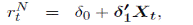 ()5
()5
 ()6
()6
where δ 0 is a constant, λ 0 and δ1 are K × 1 vectors, and λ 1 is a K × K matrix.
Assuming that the one-period log inflation rate is also an affine function of the state variables
 ()7
()7
where π 0 is a constant and π1 is a K × 1 vector, it is possible to derive the real pricing kernel
 ()8
()8
where the real short rate is
 ()9
()9
where
 and
and ; and the real price of risk is
 ()10
()10
where 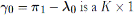 vector and
 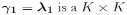 matrix.
B. Risk neutral dynamics
In the absence of arbitrage opportunities, there exists a risk neutral probability measure Q under which the state variables follow
 ()11
()11
 with , and
  . I assume that under Q, the innovations νt∗+1 are also iid Gaussian with mean
  and variance
 .
.
C. Pricing functions
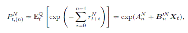
Given the above general set up, the log nominal bond price can be expressed as follows:
 .
.
By replacing the pricing kernel in Equation (4), I obtain that the coefficients are determined by the following difference equations
 ()12
()12
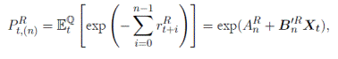
Similarly, the log price for an inflation-indexed bond is also an affine function of the state variables
 ,
,
where
 13
13
D. Unspanned liquidity factor
Duffee (2011), Joslin et al. (2014) and Boos (2011) introduce a term structure model featured by unspanned factors, which do not affect the dynamics of bonds under the risk neutral probability measure Q but do affect them under the historical measure P. The assumption that a given factor does not affect bond yields under the Q measure can be implemented by imposing the restriction that the corresponding element of  and maturities n = 1,...,h, be equal to zero (see Adrian et al., 2013).
Following Adrian et al. (2013), this restriction is incorporated by the partition of the factor vector Xt into spanned factors Xts, with nonzero risk exposure, and unspanned factor lt, which has zero risk exposure
 ,
,
where 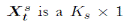 vector such that Xt is of dimension K × 1 with
  is the upper
  matrix, and are
According to Joslin et al. (2014), unspanned factors should satisfy two conditions: not being linearly spanned by the information in the joint yield curve, and having predictive power for excess returns in bond markets. To be consistent with these properties, the upper right vector  has to be equal to zero. Therefore, under the risk neutral probability measure,
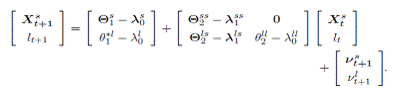
This restriction eliminates the possibility of any influence of the liquidity factor on the spanned factors; and also implies that  , so that the short rate does not load on the unspanned factor.
II. Data and factor construction
A. Data
I use daily observations on zero-coupon nominal and real Treasury bond yields constructed by Gurkaynak, Sack and Wright (2007) and Gurkaynak, Sack and Wright (2010), respectively, and obtained from the Federal Reserve website. The sample period is from January 2004 to December 2013, thus covering most of the history available for TIPS.
Given my purpose of relating the yield curve with lack of liquidity, which is a variable related to greater price uncertainty and volatility, I am not interested in monthly data, as is usual in this literature, but rather in daily yield curve data. Likewise, I am not interested in the very long-end of the yield curve (maturities above 10 years); in contrast, I am interested in a richer set of yield curve points for short- and medium-term residual maturities than those presented in Gurkaynak et al. (2007) and Gurkaynak et al. (2010). However, this dataset consists of a fitted function that smooths across maturities. In particular, what Gurkaynak et al. (2007) do is to estimate the Svennson (1994) six-parameter function for instantaneous forward rates

The parameters β0, β1, β2, β3, τ1 and τ2 are published along with the estimated zero-coupon yield curve. I use the appropriate formula and these parameters to compute the implied zero-coupon yields for a set of additional relevant intra-year maturities. I end up with a daily time series of zero-coupon yields for the 14 maturities considered in Diebold et al. (2006): 12, 15, 18, 21, 24, 30, 36, 48, 60, 72, 84, 96, 108 and 120 months. I use these yield curve data to estimate the yield curve latent factors: level, slope and curvature. However, I only use 12-, 24-, 36-, ..., 108- and 120-month nominal yields (NN = 9) and 24-, 36-, 48-, ..., 108- and 120-month TIPS yields (NR = 8) for the estimation. For this cross section, I calculate one-month holding period returns. Additionally, I use the one-month Treasury yield from Gurkaynak et al. (2007) as the nominal risk-free rate.
B. TIPS liquidity premium as unspanned pricing factor
What the literature has done for the joint pricing of the Treasury and TIPS yields is to include the TIPS liquidity as an additional spanned factor. D'Amico, Kim and Wei (2010) and Abrahams et al. (2015) model the impact of liquidity on nominal and real yields including TIPS liquidity as a spanned pricing factor. As is commonly found in this literature, D'Amico et al. (2010) use principal components extracted from TIPS yields as pricing real factors. In contrast, Abrahams et al. (2015) assume that liquidity is observed through a composite factor that measures the relative TIPS liquidity premium. It is computed as the weighted average of two observable indicators: the average absolute TIPS yield curve fitting error from the Nelson-Siegel-Svensson model of Gurkaynak et al. (2010), and the 13-week moving average of the ratio of primary dealers' Treasury transaction volumes relative to TIPS transaction volumes.
In contrast to these studies, I empirically test the plausibility of TIPS liquidity as an unspanned observed factor. I identify the liquidity component in TIPS yields through the difference between the observed break-even inflation rates and the inflation swap rates, which are considered as a synthetic BEI
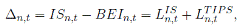 ()14
()14
Where  are the (cash BEI) break-even inflation rates, which are defined as the difference between nominal and inflation-indexed bond yields, and ISn,t
are the inflation swap rates (synthetic BEI) for the corresponding maturity n.
are the (cash BEI) break-even inflation rates, which are defined as the difference between nominal and inflation-indexed bond yields, and ISn,t
are the inflation swap rates (synthetic BEI) for the corresponding maturity n.
This measure was first used by Christensen and Gillian (2011) and combines information from the U.S. bond market with information from the inflation-indexed swaps market, which are the most liquid inflation derivative contracts traded in the OTC market.3 Christensen and Gillian (2011) argue that this difference measures the liquidity premium in inflation swaps as well as the liquidity premium in TIPS, so that it can be seen as a maximum range of liquidity premia for the TIPS market.
An important feature of zero-coupon inflation-indexed swaps (ZCIIS) is that the pricing model for nominal and inflation-linked (real) bonds would determine inflation swap rates. In fact, the first study about the pricing of ZCIIS shows that the price of inflation-indexed swaps can be expressed as a function of zero-coupon Treasury and ILBs (Mercurio, 2005).
A swap is an agreement between two counter parties in order to exchange cash flows. The agreement specifies the cash flows and the dates when they are to be paid. In particular, in a ZCIIS one party pays a fixed interest rate- commonly referred to as inflation swap rate, IS-and receives the inflation rate over the specified time period. The inflation rate is calculated as the percentage return of the consumer price index. Therefore, while the fixed payment is known at the start date of the swap, the floating payment is not. As the name indicates, a ZCIIS has only one time interval [t 0 ,T], with payments at time T and no intermediate payments.
Consider a payer of a ZCIIS that starts at time t 0 and has a payment date at time T and a swap rate equal to IS. The fixed amount (fixed leg) paid at maturity is equal to
and the floating amount received (floating leg) at maturity is
 ,
,
where It represents a price index. Then, the payoff to the holder of the ZCIIS is given by
 ()15
()15
Let Z 0(t,T,IS) denote the price of a ZCIIS at time t, t 0 < t < T. Mercurio (2005) shows that, under standard no arbitrage opportunities, the inflation-linked floating leg is equal to
 ()16
()16
where is the nominal short interest rate. But given that the nominal price of a real zero-coupon bond at time t, denoted by Pt,T
R
, equals the nominal price of the contract paying off one unit of the price index at the bond ma-
is the nominal short interest rate. But given that the nominal price of a real zero-coupon bond at time t, denoted by Pt,T
R
, equals the nominal price of the contract paying off one unit of the price index at the bond ma-
turity
 ,
,
then the price of the ZCIIS is equal to
 ()17
()17
which at time t 0 is
 ,
,
where Pt,T N is the price in dollars at time t of a nominal zero-coupon bond.
This result allows us to strip (with no ambiguity) real zero-coupon bond prices from the quoted prices of zero-coupon inflation-indexed swaps. Additionally, as Haubrich, Pennacchi and Ritchken (2012) claim, real yields on ILBs can be derived as the difference between equivalent maturity nominal yields and inflation swap rates, and these synthetic real yields are less prone to uncertain changes in liquidity than TIPS yields. For this reason, inflation swaps can be a more reliable indicator of real yields. Finally, Mercurio (2005) shows that the price of ZCIIS is model-independent, in the sense that no assumptions on the dynamics of the assets are needed to price them.
To measure liquidity, I use the market-based measure proposed by Christensen and Gillian (2011), which is defined as the difference between synthetic and cash break-even inflation rates as in Equation (14). To compute the break-even inflation rates, I use the daily estimates of zero-coupon nominal and real Treasury bond yields constructed by Gurkaynak et al. (2007) and Gurkaynak et al. (2010) from January 2004 to December 2012. For zerocoupon inflation swap rates, I use U.S. daily quotes from Barclays Live, which I convert into continuously compounded rates to make them comparable to the other interest rates. I compute this measure from January 2004 to December 2013 for an n = 10-year maturity.
C. Spanned pricing factors
As is common in the literature, I perform principal components analysis to extract the spanned pricing factors of the model from yields. Panel A of Table 1 reports the correlations between the first three principal component factors extracted from U.S. nominal Treasury yields and from TIPS yields in isolation from each other. A total number of K = KN + KR = 3 + 3 = 6 spanned model factors are computed. Table 1 shows that the pricing factors extracted from Treasuries and TIPS yields are highly correlated, exhibiting a linear correlation of 84%, 77% and 59%, respectively.
Table 1 Unconditional correlation between yield factors
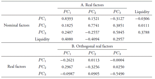
Note: panel A reports the correlations between the first three principal components for U.S. daily Treasury yields and U.S. daily TIPS yields from January 1, 2004 to December 30, 2011. Panel B reports the correlations between the first principal component from the residuals of regressions of break-even inflation rates on nominal principal components and the liquidity factor, and the first three principal components for U.S. daily TIPS yields.
Source: author's elaboration.
Consequently, I use the same two sets of principal components considered by Abrahams et al. (2015). These authors propose to extract KN = 3 principal components from nominal Treasury yields. Then, to reduce the unconditional collinearity among the pricing factors, they obtain additional factors as the first KOR = 3 principal components from the residuals of regressions of break-even inflation rates on the KN nominal principal components as well as the liquidity factor
 ()18
()18
where n = 24, 30, 36, 48, 60, 72, 84, 96, 108 and 120 months.4 These factors are called orthogonal real factors.
Table 2 shows that more than 98% of the variations in daily changes of 1-, 2-, 3-, ..., and 10-year nominal yields can be explained by the first three principal components. A similar percentage of the variation in TIPS yields, as well as in the residuals of the regressions of break-even inflation rates on nominal principal components and liquidity, can also be explained by the first three principal components. This is line with the empirical observation by Joslin et al. (2014) that bond yields follow a low-dimensional factor model, which is reflected in the fact that three factors appear to explain nearly all of the cross-sectional variation in yields.
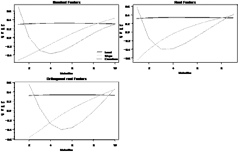
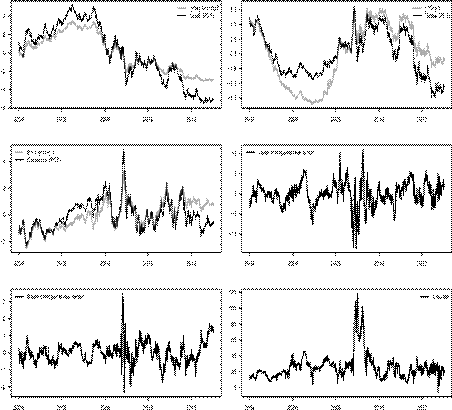
Panel B of Table 1 reports the correlations between the first three principal component factors extracted from nominal yields alone and the first three principal component factors extracted from the residuals of the regression of break-even inflation rates on nominal principal components and liquidity (i.e., orthogonal real factors). It is important to note that the first, second and third factors largely retain their interpretations as level, slope and curvature. This conclusion is based on the fact that they still have an important correlation with the first, the second and the third real factors, respectively. This is confirmed in Figure 1. As usual, each line in these graphs represents how yields of various maturities change when a factor moves. The graphs show that the level factor is almost flat, meaning that a level factor shock changes the interest rates of all maturities by almost identical amounts. The slope factor rises monotonically through all maturities, and the curvature factor is curved at the short-end of the yield curve.
Table 2 Variance explained by principal components
Note: nominal factors correspond to the first three principal components for U.S. daily Treasury yields from January 1, 2004 to December 30, 2011. Real factors correspond to the first three principal components for U.S. daily TIPS yields. Orthogonal real factors correspond to the first principal component from the residuals of regressions of break-even inflation rates on nominal principal components and the liquidity factor for the same sample period. Source: author's elaboration.
Finally, Figure 2 plots the level ( LN t ), the slope ( S t N ) and the curvature ( C t N ) nominal factor, along with the orthogonal real factors (level LOR t and slope S t OR , which correspond to the first two principal components of the residuals from Equation (18)) and the liquidity premium factor (∆ t ). Factors are constructed using principal components analysis after the data series are demeaned and divided by their respective standard deviations to make them comparable units.5 Nominal factors are plotted together with their empirical proxies: the average of short-, medium- and long-term yields for the level factor; the difference between long- and short-term yields for the slope factor, and the difference between twice medium-term yields with respect to the sum of short- and long-term yields for the curvature factor. In all cases, the principal component factors and their standard empirical proxies are closely linked. Additionally, the level and slope factors display very high persistence, while the curvature is less persistent.
III. Testing the empirical plausibility of TIPS liquidity premium as an unspanned factor
A. Testing Joslin et al.'s unspanning conditions
Following Joslin et al. (2014), the plausibility of the TIPS liquidity premium as an unspanned factor would be defined by three empirical observations: First, the TIPS relative liquidity premium is not linearly spanned by the information in the joint yield curve. Second, the unspanned liquidity factor has a predictive power for excess returns in bond markets. And third, bond yields follow a low-dimensional factor model.
To empirically test the first observation, I consider the projection of liquidity onto the principal components of yields on U.S. nominal Treasury and TIPS zero-coupon bonds, with maturities of 12 through 120 months. Results presented in Table 3 suggest that nominal Treasury and TIPS yields contain a factor that is not spanned by the traditional yield curve factors. In fact, the projection of liquidity onto the first three principal components gives an adjusted R-squared of 0.14, thus approximately 86% of the variation in liquidity is due to risks different from the traditional nominal yield factors. Similarly, the adjusted R-squared in the case of the real yield factors is about 0.42, which is much higher than in the case of nominal factors. However, 58% of the variation in TIPS liquidity can still be attributed to risks different from the real yield factors.
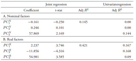
To further uncover whether the yield curve captures liquidity variation, the last column of Table 2 reports R-squared values for univariate regressions of liquidity on each yield principal component separately. Only a small portion of the variation in liquidity is captured by nominal yields; in fact, the R-squared values are zero except for the third factor. Real yields capture more variation in liquidity, however the R-squared values are all below
0.2. This is in line with Bauer and Rudebusch's (2015) explanation to the source of spanned and unspanned variation, which is based on the monetary policy reaction function. Variables that substantially drive monetary policy show very little evidence of unspanned variation and are essentially spanned by the yield curve, while those variables that display a weak relation with the policy rate and, consequently, monetary policy exhibit significant unspanned variation. This reflects the low weight these variables have in directly setting the short-term interest rate by the monetary authority, which is the case of liquidity.
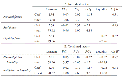
Nevertheless, results in Table 4 suggest that there exists a factor that is important for explaining the variations in TIPS yields, and also for modeling nominal interest rates. Following D'Amico et al. (2010), I regress the 10-year break-even inflation rate on the first principal components of yields
 ,
,
where i = nominal Treasury (N) or TIPS yields (R). Results show that 31% of the variation in the break-even inflation rate is explained by the first three principal components of nominal yields. Once I include liquidity in this regression, the adjusted R-squared is about 0.77. This also occurs when I consider the first three principal components of TIPS yields. In this case, the adjusted R-squared is about 0.45 and rises up to 0.73 when the liquidity factor is included. In the regression of the 10-year break-even inflation rate on the liquidity factor, the adjusted R-squared is about 0.62.
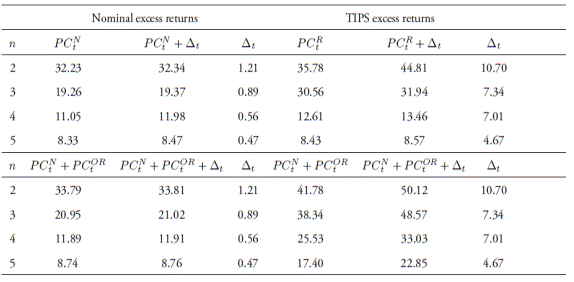
With regard to the second observation, the unspanned TIPS liquidity factor forecasts bond excess returns if liquidity significantly improves the yieldsonly forecast. To examine this, I explore whether or not the liquidity premium has considerable predictive power for excess returns over and above PCt i , where i = Nominal Treasury (N) or TIPS yields (R). Table 5 shows the adjusted R-squared values for individual bond excess returns considering the following standard predictive regression framework:
 ,
,
where  denotes annual excess log returns on n = 2-, 3-, 4-, and 5-year maturity, calculated as
 with
with  being the holding oneyear log-return on a zero-coupon n-period bond, and yt
1 is the one-year log yield.
being the holding oneyear log-return on a zero-coupon n-period bond, and yt
1 is the one-year log yield.
Table 4 Regression of break-even inflation rates onto yield and liquidity factors
Note: panel A regresses 10-year break-even inflation rate on TIPS liquidity and the first three principal components for U.S. daily Treasury yields from January 1, 2004 to December 30, 2011. Panel B regresses 10-year break-even inflation rate on TIPS liquidity on the first three principal components for U.S. daily TIPS yields using the same sample period. TIPS liquidity corresponds to the TIPS liquidity premium measure proposed by Christensen and Gillian (2011). Source: author's elaboration.
Table 5 shows the adjusted R-squared of regression forecasts with a combined set of yields and liquidity factors. The first column represents the adjusted R-squared of regressions, which includes yield factors as instruments, while the second column comprises yields and liquidity. Comparing the adjusted R-squared of regressions with the yields-only factors leads to the conclusion that the liquidity variable contains information that is unspanned by yields.6
In summary, results from the regressions presented earlier confirm that the TIPS liquidity premium, which represents the liquidity differential between U.S. Treasury and TIPS bonds, is to some extent unspanned by the nominal and real yield curves and forecast bond excess returns along with yield curve information. As a result, I find empirical evidence to suggest that the TIPS liquidity is not spanned by the yield curve, but it is important for enhancing bond return predictability. Consequently, liquidity premium could be included as an additional unspanned forecasting variable not only in forecasting regressions, but also in term structure models.
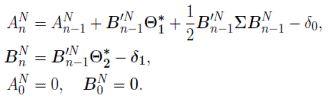
B. Estimation of the five-factor model
From the estimation of the five-factor Gaussian term structure model presented in Section II (including four principal components of zero-coupon yields, plus the liquidity premium as pricing factors), I am interested in testing for the presence of unspanned factors. I do so by checking whether or not particular columns of B′ are equal to zero. Let b i be a particular column of B′. Then, based on the asymptotic distribution of the factor risk exposures B′ derived by Adrian et al. (2013), and under the null hypothesis Ho: b i =
0 N ×1, the Wald statistic is given by
 ,
,
Table 5 Adjusted R-squared values
Note: panel A regresses 10-year break-even inflation rate on TIPS liquidity and the first three principal components for U.S. daily Treasury yields from January 1, 2004 to December 30, 2011. Panel B regresses 10-year break-even inflation rate on TIPS liquidity on the first three principal components for U.S. daily TIPS yields using the same sample period. TIPS liquidity corresponds to the TIPS liquidity premium measure proposed byChristensen and Gillian (2011).Source: author's elaboration.
with ΥB = σ 2(I⊗ Σ−1 ). I start by assessing the relative importance of each of the model factors in explaining the cross-sectional variation of nominal Treasury returns, TIPS returns, and their joint cross section.
Table 6 provides the Wald statistics and the associated p values for tests of whether or not the risk factor exposures associated with individual pricing factors are jointly different from zero. As indicated by the associated Wald statistics in the first column of Table 1, nominal Treasury returns are significantly exposed to all three principal components extracted from nominal Treasury yields as well as to the first principal component extracted from orthogonalized break-even. However, I do not reject the null hypothesis that the liquidity factor has zero B. Similarly, TIPS returns co-move strongly with innovations to all traditional spanned pricing factors of the model. However, this is not the case for the liquidity premium factor. Moreover, considering the joint cross section of nominal Treasury and TIPS returns, I find that the liquidity factor is not associated with significant risk exposure. These findings are in line with the empirical evidence presented before and justify the assumption of treating the liquidity premium factor as unspanned in the specification.
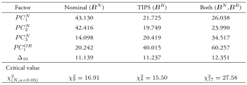
Table 7 Market prices of risk: unspanned specification
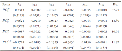
Note: nominal factors PCt N correspond to the first three principal components for U.S. daily Treasury yields from January 1, 2004 to December 30, 2011. Orthogonal real factors PCt OR correspond to the first principal component from the residuals of regressions of break-even inflation rates on nominal principal components and the liquidity factor for the same sample period. Liquidity premium unspanned factor ∆ 10,t corresponds to the measure proposed by Christensen and Gillian (2011) for the liquidity differential between TIPS and nominal Treasury yields. Standard errors are reported in parenthesis. Source: author's elaboration.
Finally, liquidity is the only factor that significantly affects the market price of the curvature risk. This result can be interpreted as indicating that the information contained in the yield curve is insufficient to completely characterize the variation in the price of curvature risk. This result is somewhat consistent with the results in Abrahams et al. (2015), who find that the liquidity factor significantly affects the market price of the curvature risk as well as that of the liquidity risk. However, these authors consider liquidity as an additional spanned factor.
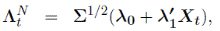
To summarize the pricing implications of the model, I test the null hypothesis that the different rows of Λ, which includes λ0.i
and λ1.i
and is denoted by  , are equal to zero. Then the corresponding Wald test for the
Ho: λ′ i = 01×( K+1) is given by
 .
.
The last column in Table 7 provides the Wald statistic values.7 I find that the level and slope risks are priced in the five-factor model. This is not a surprising result given that the level and slope risks capture the first and second largest share of the cross-sectional variation of yields. However, the curvature risk appears not to be priced at α = 5%, although most of the individual elements of λ 1 (for the second row of λ) are significantly different from zero. The orthogonal level factor, as measured by the exposure to the first principal component from the residuals of regressions of break-even inflation rates on nominal principal components and the liquidity factor, is priced in the model.
C. Does the variation in TIPS liquidity premium forecast the yield curve factors?
In the affine model (Section A), the assumption that the liquidity factor is unspanned was implemented by imposing that the upper right vector  be equal to zero under the risk neutral probability measure. This restriction eliminates the possibility of any influence of the liquidity factor on the spanned factors under Q, but it has predictive ability for the future evolution of the yield curve factors. In other words, it has predictive information for the yield curve factors as Joslin et al. (2014) pointed out.
As an additional test to determine whether the liquidity factor is truly unspanned by the yield curve, I examine in this section the empirical relation between movements in the level, the slope and the curvature of the term structure of U.S. nominal and real interest rates, and the TIPS liquidity premium shocks. I infer the relation between yield movements and shocks on the liquidity premium using IRFs implied from a VAR model.
The VAR model is estimated with the principal components formed from the set of nominal and TIPS yields described in Section II. I order the term structure factors prior to the TIPS liquidity premium variable as follows: LN t , St N, Ct N, LOR t , St OR , and ∆ t .8 The number of lags in each VAR is chosen using the same set of informational criteria used before, with the minimum lag suggested by the four criteria being equal to 2.
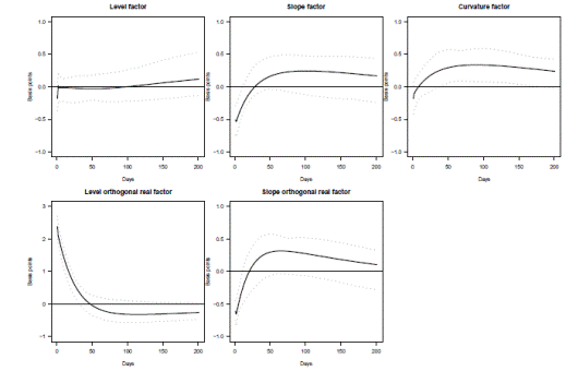
Figure 3 illustrates the response of a particular variable to a unit standard deviation change in the TIPS liquidity premium traced forward over a period of 200 days. In other words, the graphs depict the effect of a one-time shock to liquidity on the current and future value of the particular span yield factor. Dashed lines represent bootstrap 95% confidence bands derived via 1,000 bootstrap simulations.
The first graph in Figure 3 presents the impulse-response function for the level nominal factor. The result indicates that the level factor first increases in response to a one-standard deviation shock to liquidity; but then it starts to decrease a few days after the initial shock, becoming negative thereafter. This result indicates that an increase in the TIPS liquidity premium affects the overall level of nominal interest rates, shifting down the yield curve. In other words, under increased TIPS liquidity risk, demand for all nominal bonds would increase, which would lead to an overall increase in nominal bond prices, thus decreasing rates of all maturities and leading to a downward shift in the yield curve. The second graph shows that the effect of a one-standard deviation shock to the TIPS liquidity is positive for the slope

factor, meaning that it makes the yield curve steeper. Thus, when liquidity conditions worsen in the TIPS market relative to the nominal market, nominal long-term interest rates change by much larger amounts than short-term rates. The effect persists for at least one year, being the cumulative slope impact approximately equal to 1.06% in the first year. The curvature factor also increases in response to a liquidity shock, as the third graph shows, which indicates that the yield curve becomes more curved at the short end. The effect is persistent, however a shock to liquidity appears not to have a significant impact on any of the nominal factors.
With regard to real factors, the fourth graph reveals that a shock to the TIPS liquidity premium predicts an important negative current impact for the orthogonal real level factor, with this impact gradually increasing toward zero after the initial shock. The contemporaneous effect is about −0.15%, meaning that a one-standard deviation shock to liquidity decreases the orthogonal real factor by 0.15 percentage points. In other words, if the liquidity premium rises by 16.55 basis points, the general level of real interest rates would lower by 0.15%. Finally, the fifth graph illustrates the response of the orthogonal real slope factor to a unit standard deviation change in the liquidity premium. The slope real factor rises in response to a liquidity shock, with the response decaying slowly.
Figure 4 provides the response of liquidity to perceived changes in the nominal and real yield traditional factors. In this figure, the responses give the basis points change in the liquidity premium to a one-standard deviation shock to yield factors.9 The first graph displays the impulse response to a level shock. The level shock has an initial negative impact on the relative liquidity of TIPS with respect to nominal bonds, with the immediate impact being a decrease of about −20 basis points (−0.2). The liquidity response turns positive after about four months.
While the estimated impulse responses of liquidity to a level shock are mostly insignificant, they are economically meaningful. In fact, the level factor (or general level of interest rates) has been associated with the bond market's perception of the long-run inflation rate by several studies that have explored macroeconomic influences on the yield curve (see Dewachter & Lyrio, 2006; Diebold et al., 2006; Rudebusch & Wu, 2007, among others). Under this interpretation, an increase in the level factor (i.e., an increase in future perceived inflation) generates an expectation of higher inflation risk, which lowers the (ex-ante) real interest rate. This may increase the demand of TIPS, which in turn increases the price of those bonds while simultaneously causing yields to decrease. Thus, the yield gap between TIPS and nominal Treasury bonds becomes wider, reflecting the persistent inflation concerns of the market and also potential changes in liquidity conditions. Additionally, an increase in the level factor raises the federal funds rate (FFR), which is related to a tightening of monetary policy. However, during the sample period considered in this paper, the Federal Reserve has accommodated only a small portion of the expected rise in inflation. In contrast, the federal funds target has been as low as it can be since 2008, fixed by the Fed at zero lower bound.
Furthermore, even before the financial downturn began in 2007 real interest rates had fallen sharply, especially over the previous six years. One direct consequence of low real interest rates is that bond returns (and, in general, asset returns) are expected to be highly volatile. In fact, when the real interest rate is unusually low, asset prices become sensitive to information about dividends or risk premia in the distant future (Kocherlakota, 2014). This in turn causes an increment in the TIPS liquidity risk premium.
A shock to the slope factor has a negative initial impact on the liquidity premium, starting to increase and becoming positive approximately 30 days after the initial shock. In fact, a one-standard deviation shock to the slope factor results in an initial decrease in liquidity of about 51.66 basis points. Similarly, the TIPS liquidity premium responds negatively to an increase in the curvature factor. In this case, the TIPS liquidity premium decreases initially by approximately 18.71 basis points. After that, the liquidity premium rapidly increases, becoming positive after a few days, and reaches its maximum level two months after the initial shock.
The slope factor (or tilt of the yield curve) has been related to monetary policy actions, and particularly to future interest rate movements. Diebold et al. (2006) show that there is a close connection between the slope factor and the instrument of monetary policy, the FFR. Their hypothesis is that if the Federal Reserve pursues an expansionary monetary policy (dropping the rate), the increase in funds could cause higher order inflows into nominal government bonds and potential changes in their liquidity conditions. In other words, decreases in the FFR (a looser monetary policy) would increase liquidity because of the reduction in the financing cost. It is natural to think that the liquidity risk for TIPS is correlated with the small liquidity risk that exists for nominal Treasury notes. It is also widely accepted that if there is a small liquidity risk associated with holding nominal Treasury bonds, there is an even larger liquidity risk associated with holding TIPS. Consequently, decreases in the FFR would increase liquidity in both markets, which means a reduction of the liquidity premium demanded by investors to hold TIPS, given the decrease in liquidity risk.
The sample period under analysis includes the last financial crisis and the Federal Reserve's unprecedented response to it. In the first half of 2004, the Federal Open Market Committee (FOMC) was particularly attentive to the possibility that economic growth accelerated unexpectedly, leading to inflationary pressures. Despite judging those pressures as temporary, the FOMC tightened monetary policy by increasing the federal funds target. Later, in a series of 10 moves, the target was reduced from 5.25% beginning in September 2007 to a range of 0% to 0.25% on 16 December 2008 as a response to the unusually severe crisis. Before 2008, short-term interest rates had never reached the zero lower bound. However, rates remained there for several years after that. With the federal funds target at the zero lower bound, the Federal Reserve attempted to provide stimulus through unconventional policies such as quantitative easing, a program by which the government buys large quantities of illiquid assets in order to affect their prices and yields. Even so, the largescale asset purchase (LSAP) program appeared to improve market liquidity in general. Christensen and Gillian (2011) show that the second round of the LSAP program helped to improve the TIPS market functioning on purchase dates, and throughout the program, by reducing the liquidity premia that investors would have demanded had the purchases not been conducted. The observed events over the sample period suggest that under overall uncertainty in the market, the TIPS liquidity premium has not responded to conventional monetary policy actions such as a lowering of the federal funds rate, but instead it has decreased in response to unconventional policies.
Finally, a one-standard deviation shock to the orthogonal real level factor forecast has a large positive effect on the liquidity premium on impact, starting to decrease and becoming negative (essentially in a permanent way) after 50 days of the initial shock. In particular, following an increase of one standard deviation in the real factor, the liquidity differential between Treasuries and TIPS yields increases by approximately 238 basis points initially. After that, the liquidity differential starts to decrease, being mostly significant within the first two months. Finally, the TIPS liquidity premium responds in a similar way to a one-standard deviation shock to the real slope factor. The initial effect is negative, starting to rapidly increase and becoming positive approximately 20 days after the initial shock.
Summarizing, the TIPS liquidity premium influences the shape of the joint nominal and real yield curve. It has an economically significant impact on nominal yield factors, and also a statistically significant effect on real factors. Conversely, shocks to nominal and real bond yield factors appear to have an effect on the liquidity premium. This effect is meaningful given that, as previous empirical evidence has shown, the yield curve factors are highly correlated with measures of inflation expectations and monetary policy instruments, which provides an explanation for this dynamic connection.
Conclusion
In this paper, I consider a joint Gaussian affine term structure model for zero-coupon U.S. Treasury and TIPS bonds, with an unspanned factor consisting of liquidity risk. The liquidity factor is restricted to affect the cross section of yields but it is allowed to determine the bond risk premia. In other words, I am considering liquidity as an additional factor that does not span the yield curve but improves the estimation of bond risk premia. I use different sources of data (nominal Treasury yields, TIPS yields and inflation swap rates) to estimate the parameters of the model. In particular, I use information on zero-coupon inflation swaps to identify the physical liquidity risk premium, which arises from the liquidity differential between Treasuries and TIPS bonds.
In the context of this empirical model, my first conclusion is that the TIPS liquidity premium is indeed an unspanned factor that helps to forecast U.S. bond risk premia, and that it is not linearly spanned by the information in the joint yield curve. Second, I show that the variation in the TIPS liquidity premium influences the shape of the yield curve in the sense that it predicts the future evolution of the traditional yield curve factors. In fact, an increase in the TIPS liquidity premium lowers the nominal interest rates of all maturities. Similarly, the effect of a one-standard deviation shock to TIPS liquidity is positive for the slope factor, meaning that it makes the yield curve steeper. Thus, when liquidity conditions worsen in the TIPS market relative to the nominal market, nominal long-term interest rates change by much larger amounts than short-term rates. The curvature factor also increases in response to a liquidity shock, which indicates that the yield curve becomes more curved at the short end.
Third, I conclude that the liquidity factor significantly affects the market price of curvature risk only. This result can be interpreted as indicating that the information contained in the yield curve is insufficient to completely characterize the variation in the price of curvature risk. This result is somewhat consistent with the results in Abrahams et al. (2015), who find that the liquidity factor significantly affects the market price of curvature risk, as well as that of liquidity risk, when liquidity is considered as an additional spanned factor. I leave for future work consideration of additional unspanned factors (such as real output and inflation), and to perform out-of-sample exercises in order to compare different factor model specifications.
Finally, there is evidence of potential mispricing in the TIPS market. In fact, Treasury bonds have been consistently overpriced relative to TIPS. This raises doubts about whether a no-arbitrage framework is adequate to model TIPS yields and obtain risk premia from it. Nevertheless, the empirical model in this paper is still of interest as it provides a baseline factor structure for the yield curve. In future research, it would be interesting to consider a more general setting. Improving our understanding of TIPS might potentially help to employ these securities more efficiently both from a policy and an investors perspective.

