


 English (pdf)
 Article in xml format
 Article references
 Send this article by e-mail
 Cited by SciELO
  Cited by Google
  Similars in
SciELO
Similars in
SciELO  Similars in Google
 Permalink
Introduction
The interbank funds market plays a central role in monetary policy transmission, as it allows financial institutions to exchange central bank money in order to share liquidity risks (Fricke & Lux, 2014). For that reason, they are
the focus of central banks' implementation of monetary policy and have a significant effect on the whole economy (Allen, Carletti, & Gale, 2009; p. 639). In addition, the absence of collaterals in the interbank funds market creates powerful incentives for participants to monitor each other, and thus it plays a key role as a source of market discipline (Rochet & Tirole, 1996; Furfine, 2001). Therefore, the interbank funds market is an important element for an efficiently functioning financial system (Heijmans, Heuver, & Walraven, 2010).
Reliable and comprehensive data from the interbank funds market is somewhat elusive, with restrictions on the consistency, granularity, and opportunity of the corresponding databases. This explains the numerous research articles that aim at identifying unsecured (i.e., non-collateralized) interbank funds loans from large-value payment systems' transactional data. The first of such articles is credited to Furfine (1999), who developed an algorithm for identifying interbank overnight loans for the US money market from Fedwire data. The procedure in Furfine (1999) is straightforward: matching payments in day t from Bank A to Bank B greater than one million dollars rounded to the nearest integer of $100,000 (i.e., the loans), with payments from Bank B to Bank A in day t +1 (i.e., the overnight refund) such that the implicit interest rate between both payments is reasonable (i.e., it falls inside a ±50 basis points corridor with respect to publicly available measures of the federal funds rate). This general approach is commonly referred as Furfine's method or Furfine's algorithm.
After Furfine (1999) several authors have attempted to apply similar algorithms. Demiralp, Preslopsky, and Whiteshell (2004) include smaller size loans (i.e., greater than $50,000, with equal-sized increments) and include an interest rate 1/32-rounding rule for discarding interbank overnight transactions that are incompatible with market practices. Millard and Polenghi (2004) apply Furfine's algorithm to UK's large value payment system (CHAPS), including a threshold on one million pounds. Hendry and Kamhi (2007) apply Furfine's algorithm to data from the Canadian large value transfer system with a half a basis point rounding rule for filtering transactions. Some authors have considered interbank non-overnight transactions for the Dutch, Swiss, and Euro interbank markets (see Heijmans et al. 2010; Guggenheim, Kraenzlin & Schumacher, 2011; Arciero et al., 2013).
Regarding the validity of the Furfine's method, Armantier and Copeland (2012) have questioned the results obtained when implementing Furfine's method. On the other hand, Arciero et al. (2013) contrast results reported by Armantier and Copeland, and confirm the validity of Furfine's method conditional on a deep knowledge of the underlying data and the technical attributes of the system under analysis.
This paper implements the Furfine's method on an unusual dataset from the unique Colombian large-value payment system (Cuentas de Depósito - CUD). As explained in detail below, it is an unusual dataset because loans and refunds may be easily and accurately filtered out from large-value payment system's raw data. Our objectives are the following: First, to filter out interbank funds transactions in the Colombian market in order to identify loans of all maturities (up to 90 days) without relying on data reported by financial institutions;2second, to contrast the loans identified by our algorithm with those identified from reports by financial institutions, and to contrast our implicit interbank overnight interest rate (IIRON ) with the publicly available interbank overnight reference rate (IBRON ) and interbank overnight funds average rate (TIB); and third, to construct the interbank claims networks, a key input for examining financial contagion under recent approaches to systemic risk and financial stability.
By accomplishing these three objectives, we expect to provide evidence on the usefulness of large-value payment systems' data for monitoring, overseeing, and analyzing the interbank funds market. Some uses are worth emphasizing. First, as this type of exercise provides the opportunity to evaluate the interbank funds market without relying on reports from financial institutions, lags and potential errors arising from consolidating, processing and transmitting reports by financial institutions and financial authorities may be conveniently avoided. As financial authorities have to rely on delayed and costly sources of data (i.e., reported data, on-site and off-site analyses), it is warranted to have potential alternatives (Kyriakopoulos et al., 2009).
Second, transactional data grants financial authorities the ability to contrast surveys and reports by financial institutions. As the Libor panel scandal demonstrated (see Guggenheim et al., 2010), the ability to contrast is rather limited when relying on reports and surveys only.3 Also, as stressed by Kyriakopoulos et al. (2009), using financial transaction records is particularly useful to uncover financial misconduct and rogue trading.
Third, using transactional data allows monitoring the interbank overnight funds market in a continuous manner. Therefore, as suggested by Heijmans et al. (2010), it should be used as an early warning indicator tool, both at the macro level (the whole market) and at the individual (financial participants) level.
It is important to state that our implementation of Furfine's method is somewhat easier than in other markets. Interbank transactions settled in large-value payment systems are not labeled as such in most systems around the world (Heijmans et al., 2010), whereas the Colombian large-value payment system obliges financial institutions to use specific codes when registering interbank transactions. Before March 2013 there was a single code for interbank funds transactions, which did not allow distinguishing between loans and refunds. After March 2013, separate codes for intraday and nonintraday loans and refunds were enacted. Therefore, unlike most attempts to implement Furfine's method, our dataset is unusual as we already have identified loans and refunds, and our task is to match converse transactions at a reasonable implicit rate in the future. As described below, such matching requires defining an area of interest rate plausibility (i.e., an interest rate corridor) with respect to publicly available interbank reference rates, defining a procedure for solving multiple refund matches for a single loan, and defining transactions' maximum reliable time to maturity.
Three main contributions are worth stating. First, consistent with the lack of timely and granular information during the Great Financial Crisis, we provide further evidence on the usefulness of large-value payment systems' data for monitoring, overseeing, and analyzing the interbank funds market. Second, we emphasize the importance of recent efforts by financial authorities to attain detailed financial transactions datasets (e.g., Bank of England, 2015);4that is, turning our rather unusual dataset into a standard is now deemed advantageous for implementing monetary policy and financial stability. Third, by running the algorithm backwards (i.e., starting with the last date of the sample until reaching the first one) we attained a practical method for mitigating the over-identification of long-term interbank loans, an issue also encountered by Guggenheim et al. (2010) and Heijmans et al. (2010).5 To the best of our knowledge, this backwards-run setup has not been attempted in related literature before, and may be worth exploring in further implementations of Furfine's algorithm.
I. The Dataset
As usual in other implementations of Furfine's method, the data source is the local large-value payment system. This method relies on the premise that all interbank loans will eventually result in a converse payment between financial institutions in the large-value payment system. Such premise may be questionable whenever financial institutions tend to settle their interbank transactions outside the large-value payment system, say on the books of a common settlement bank, or by the physical delivery of cash or checks between them.6
In Colombia, there is a single large-value payment system (CUD), which is owned and operated by the Central Bank (Banco de la República). This is the financial market infrastructure where all cash settlements (in local currency) take place, for all types of financial transactions -including interbank funds transactions. All types of financial institutions, banking and non-banking, local and foreign-owned, private and government-owned, are allowed to directly participate in the large-value payment system; that is, this is a non-tiered payment system with no settlement banks.
To the best of our knowledge, there is no information about the significance of interbank loans and refunds settled outside the local large-value payment system. We presume that the non-tiered access scheme of the Colombian large-value payment system, and the corresponding absence of settlement banks, should make the settlement of transactions in the books of a common financial institution unnecessary -therefore rare. However, as there are no limitations to these kinds of external settlements, or to the settlement of transactions by the physical delivery of cash or checks, we cannot rule out that some interbank loans and refunds are settled outside the largevalue payment system. All in all, we expect external settlements of interbank loans and their refunds to be unimportant.
The local large-value payment system obliges financial institutions to classify their transactions based on a set of codes determined by the Central Bank. Regarding the interbank funds market transactions, after March 2013 financial institutions use distinct codes for registering interbank loans and refunds when executing the transfer of funds. Nonetheless, there is no tracking or earmarking between each loan and its corresponding refund.
Financial institutions do not register all interbank funds transactions in the large-value payment system. Interbank funds transactions corresponding to the interbank reference rate formation program (Índice Bancario de Referencia- IBR) are registered in the large-value payment system by a second financial market infrastructure, Depósito Central de Valores (DCV), which is the securities settlement system and the central securities depository for sovereign securities.
Hence, unlike most implementations of Furfine's method, the dataset is already filtered out. All non-interbank funds transactions may be easily discarded, and the remaining data are already classified as a loan or as a refund. The dataset consists of all interbank funds transactions between 1 April, 2013 and 30 December, 2014 (i.e., 428 business days); so intraday interbank transactions are not considered. This dataset comprises 27,200 interbank funds transactions: 13,504 correspond to interbank transactions registered by financial institutions directly, whereas 13,696 correspond to interbank transactions registered by DCV on behalf of the interbank reference rate formation program. The value of the interbank transactions corresponding to the reference rate formation program (i.e., registered in CUD by DCV) represents about 21.6% during the period under analysis.
Some features shape the Colombian interbank market. As with the largevalue payment system, direct access is open to all types of financial institutions (i.e., banking and non-banking, local and foreign-owned, private and government-owned); that is, it is a bilateral, non-brokered, interbank market. Nevertheless, only a fraction of banking institutions lends and borrows in the interbank market on a regular basis. Most financial institutions, typically small in size, lend and borrow against collateral only. Accordingly, the contribution of unsecured borrowing to total borrowing between financial institutions is rather low, about 9.68% (see Banco de la República, 2015).7 Hence, as reported by Martínez and León (2015), the Colombian interbank market appears to be a case of liquidity cross-underinsurance (see Castiglionesi & Wagner, 2013), in which strong negative externalities arising from counterparties' failure creates incentives not to provide liquidity in the absence of collateral or any other guarantee scheme.
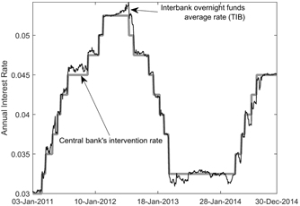
Both the interbank overnight funds average rate (TIB) and the target rate for implementation of Central Bank's monetary policy display a strong linear dependence, resulting in a 0.99 correlation for the 2011-2014 period. Also, the average absolute difference between these two rates is about 5 basis points, whereas the maximum absolute difference is 30 basis points. Therefore, as exhibited in Figure 1, the interbank overnight funds rate follows Central Bank's rates closely -as intended by monetary policy.
II. The algorithm
Unlike Furfine (1999) and most of the related literature on Furfine's method, due to the unusual features of our dataset, our algorithm does not filter interbank transactions out from (raw) large-value payment data. Such features of the dataset avoid us making some assumptions for identifying loans and refunds. For instance, following the algorithm's setup by Arciero et al. (2013), we do not need to define minimum loan values and increments in loan values to filter out potential loans. As making such assumptions is critical for minimizing false negatives and false positives (Arciero et al., 2013), working with filtered data should mitigate some serious sources of error.
Yet, some steps in the setup of the algorithm remain: First, defining the implicit interest rates' plausibility (i.e., the interest rate corridor); second, excluding plausible rates that do not conform to market practices; third, defining a solution procedure in case of multiple refund matches for a single loan; and fourth, defining the transactions' maximum reliable time to maturity.
Regarding the first remaining step, as not all financial institutions can trade liquidity at the same rates, an area of plausible interest rates has to be defined (Heijmans et al., 2010). Related literature favors a symmetrical or quasi-symmetrical corridor around a representative publicly available interbank rate. For instance, for the US Furfine (1999) uses a corridor of 50 basis points below (above) the minimum (maximum) of each day's federal funds' 11:00 rate, closing rate, and value-weighted funds rate. Demiralp et al. (2004) uses a wider ±100 basis points corridor with a minimum rate of 1/32. Heijmans et al. (2010) use a ±100 basis points corridor with respect to Eonia (European Overnight Index Average) and Euribor throughout the European Central Bank's liquidity injection and interest rate decrease (i.e., September 2008-September 2009), and a ±50 basis point corridor for the rest of their sample. Arciero et al. (2013) use three corridors (±25, ±50 and ±200 basis points) with respect to Eonia.
The area of plausibility should be chosen in such a way that it minimizes the probability of Type 1 and Type 2 errors (Heijmans et al., 2010). Type 1 error results when a transaction is mistakenly identified as an interbank transaction (i.e., a false positive), whereas Type 2 error results when an interbank funds transaction is erroneously omitted (i.e., a false negative). In our case the occurrence of Type 1 error is low due to the features of the dataset (i.e., interbank funds transactions only). As for Type 2 error, omitting actual interbank funds transactions may result from the choice of the area of plausibility: The narrower the corridor, the more likely it is to misclassify actual interbank funds transactions as implausible.
As in our case the occurrence of Type 1 error is expected to be low due to the features of the dataset, choosing a significantly wide area of plausibility may definitely minimize Type 2 error. However, a wide corridor may cause a Type 3 error, in which the algorithm yields a "wrong match" from multiple matches (see Arciero et al., 2013). Therefore, a too lax plausibility area is to be avoided as it may result in an unwarranted recurrence of multiple potential refund matches for a single loan.
Akin to Arciero et al. (2013), we use several corridors in order to test whether the results, along with the occurrence of Type 2 and 3 errors, are robust to the change of plausibility area. We use three corridors of ±50, ±100 and ±200 basis points with respect to the maximum and minimum publicly available interbank reference rates (IBR) for the overnight, one-month and three-month time to maturities. A minimum plausible interest rate is set at 1.00 %.
As for solving for multiple potential matches, we use a recursive procedure. In case two or more potential refunds are available as plausible matches for a single loan, the algorithm estimates the interbank funds market term structure for all maturities from overnight to 90 days based on the three available interbank reference rates (i.e., overnight IBR, one-month IBR, and threemonth IBR). The estimation of the term structure is done by cubic spline interpolation. The resulting term structure is used as a benchmark for deciding which of the competing plausible rates is the closest in absolute terms (i.e., lowest absolute spread) to the interpolated market price for liquidity. Afterwards, if two or more potential refunds persist, the one with the lowest time to maturity is chosen. This is consistent with interbank funds market maturities in the Colombian case, in which most transactions take place in the very short term, usually overnight. Finally, if the competing plausible refunds share the same absolute difference with respect to the interbank funds term structure, and have the same time to maturity, we use a first in first out (FIFO) rule that privileges the first occurring refund in the day.
Finally, we determine the maximum reliable time to maturity for the loans. Data from the Financial Superintendency disclose that the maximum time to maturity reported by financial institutions is 35 days during the period under analysis, in May 29, 2013. Therefore, one of our scenarios consists of limiting the maturity of potential refunds to 35 days. However, as one the advantages of using transactions data is to contrast other sources of information, and because longer maturities occurring in the future should not be disregarded, we also use a 90-day maximum reliable time to maturity scenario. Comparing both maturity scenarios will be useful for testing whether the algorithm is robust to different specifications.
Note that in designing the setup of the algorithm we do not consider excluding plausible rates that do not conform to market practices. This is a step that uses market practices or anecdotal evidence (e.g., rounding rules, minimum loan values, typical increments in value) to discard implausibly complicated loans or interest rates that do not follow standard interbank funds transactions (see Arciero et al., 2004; Demiralp et al., 2004). As before, because in our case the dataset is limited to interbank funds transactions, such exclusion procedure is unwarranted.
III. Main results
The main results of the implementation of Furfine's method for the Colombian interbank funds market are presented in three subsections. The first subsection compares the results obtained with different scenarios of plausible interest rates (i.e., corridors) and different transactions' maximum reliable time to maturities. After selecting the most convenient scenario for analytical purposes, the second subsection contrasts the resulting identified loans with those identified from financial institutions' reported data. The third subsection contrasts our implicit interbank overnight interest rate (IIRON ) with the publicly available interbank overnight reference rate (Índice Bancario de Referencia Overnight - IBRON ) and interbank overnight funds average rate (Tasa Interbancaria - TIB). The last subsection presents a sample of the interbank claims networks available as a byproduct of the algorithm.
A. Examining the scenarios
Six different scenarios are designed to examine the algorithm and its robustness to its setup. Different choices of plausible interest rates (i.e., the corridor) and transactions' maximum reliable time to maturities are considered for the following scenarios:
S (50|90): ±50 basis points corridor, 90-day maximum maturity
S (100|90): ±100 basis points corridor, 90-day maximum maturity
S (200|90): ±200 basis points corridor, 90-day maximum maturity
S (50|35): ±50 basis points corridor, 35-day maximum maturity
S (100|35): ±100 basis points corridor, 35-day maximum maturity
S (200|35): ±200 basis points corridor, 35-day maximum maturity
The algorithm was run forwards, starting with transactions occurring in April 1, 2013, day by day, through December 30, 2014. Although our dataset covers the period April 1, 2013-December 30, 2014, we discard some observations at the end of the sample when comparing among scenarios. As the first three scenarios consider a 90-day maximum time to maturity, comparisons will correspond to April 1, 2013-September 30, 2014 period (i.e., the last 3 months of observations are discarded). All rates are annualized rates with an actual/365 day-count convention.8 A lower bound for the corridor is set to 1.00% in all scenarios.
Table 1 compares how the scenarios matched actual transactions (by number of transactions and their value), and presents how they differ in terms of implicit interest rates and maturities.
Table 1 shows that the number and value of transactions matched from the large-value payment system's data are rather representative, slightly above 83% and 89%, respectively. Interestingly, changes in the interest corridor and the maximum reliable maturity do not affect the number and value of matched transactions: increasing the corridor by 150 basis points and the maximum reliable maturity by 55 days results in a (negligible) 0.35% and 0.60% increase in the number and value of matched transactions. This points out that some traits of the data may explain the fraction of transactions that could not be captured by the algorithm. These traits may include the separate refund of principal and interests; the aggregation of two to more refunds into a single settlement; and the settlement of the loan (or the refund) outside the largevalue payment system (e.g., by the physical delivery of cash or checks).
Table 1 also shows that the main overall outcomes of the algorithm are rather robust to its setup. There are trivial differences in the number and value of transactions matched from actual data, in the average implicit interest rates, and in the average time to maturities. However, there are non-negligible differences in the range (i.e., from minimum to maximum) of implicit interest rates and time to maturities. Moreover, all scenarios corresponding to the 90day maximum reliable maturity tend to over-identify transactions, especially when the corridor widens. For instance, although the maximum observed time to maturity reported by the Financial Superintendency for the period under analysis is 35 days, the first three scenarios identified interbank funds transactions at maturities of 49, 85 and 90 days, in which the wider the corridor the longer the maturity. This concurs with Arciero et al.'s (2013) statement about how the amount of noise (i.e., falsely identified loans) tends to increase with the selected maximum reliable maturity. Again, as emphasized by Arciero et al., a deep knowledge of the underlying data and technical details of the system is essential to avoid spurious results.
Table 1 Comparison of selected scenarios
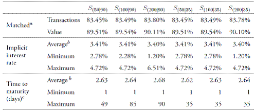
Note: a Matched transactions and matched value correspond to the number of actual transactions and value of transactions (in percentage) that are identified by the algorithm, respectively. b Simple average. c Calendar days. Source: authors' calculations.
To examine the robustness of the algorithm to its setup, we attempted a straightforward test. As mentioned, the algorithm was run forwards, meaning that we start matching interbank loans occurring in April 1 with all refunds happening after April 1, then matching loans occurring in April 2, until -recursively- reaching the last date of our sample (i.e., September 30, 2014). If the maximum reliable time to maturity is 90 days, this type of procedure allows the algorithm to try to match April 1's loans with all refunds occurring between April 2 and July 1, even though most of these refunds correspond to loans originated well after April 1. That is, by running the algorithm forwards the bulk of potential refunds corresponds to loans that occurred after April 2, and thus we should expect to be over-identifying longterm interbank loans (see Guggenheim et al., 2011; Heijmans et al., 2010).
Put another way, when run forwards the algorithm works with the sum of the distribution of refunds for each day within the maximum reliable time to maturity, with the resulting distribution of refunds departing from the observed distribution of loans time to maturity. Hence, the algorithm is forced to find matches from a set of refunds that is mostly constituted by refunds corresponding to loans occurring afterwards. On the other hand, when run backwards, starting with the last date of the sample until reaching the first one, the algorithm will try to find matches from a set of refunds that has already been used to match other loans, thus its distribution should be closer to loans observed time to maturity.9
In short, we start matching loans contracted in September 30, 2014 with the refunds registered after that date; afterwards, we match the loans contracted in September 29, 2014 with the refunds registered and available (i.e., not already matched before) after that date; and so on until reaching the first day of the sample (April 1, 2013). By running the algorithm backwards, shortterm matches will be more likely because spurious long-term potential refunds will tend to be scarce as they were already matched by short-term plausible transactions. Hence, running the algorithm backwards should mitigate the over-identification of long-maturity transactions and of false positives (i.e., Type 1 error), whilst the results should converge to those attained by defining an adequate maximum reliable time to maturity.
The backwards scenarios will be identified as follows:
Z (50|90):backwards, ±50 basis points corridor, 90-day maximum maturity
Z (100|90):backwards, ±100 basis points corridor, 90-day maximum maturity
Z (200|90):backwards, ±200 basis points corridor, 90-day maximum maturity
Z (50|35):backwards, ±50 basis points corridor, 35-day maximum maturity
Z (100|35):backwards, ±100 basis points corridor, 35-day maximum maturity
Z (200|35):backwards, ±200 basis points corridor, 35-day maximum maturity
The backwards-run scenarios in Table 2 exhibit some interesting features. First, as before, the number and value of transactions matched from the large-value payment system's data are rather representative, slightly above 83% and 89%, respectively, and they are robust to changes in the setup of the algorithm. Second, the main outcomes of the scenarios are robust in cross-section, with trivial differences in the average implicit interest rates, average time to maturity, minimum time to maturity, and number and value of captured transactions. Third, concurrent with forwards-run scenarios in Table 1, the widest corridor (±200 basis points) results in non-negligible differences in the maximum and minimum implicit interest rates, and the maximum maturities. Fourth, as expected, the over-identification of longmaturities is mitigated in the backwards-run scenarios: Z (50|90) and Z (100|90) result in a maximum time to maturity equal to that reported by the Financial Superintendency for the sample under analysis (i.e., 35 days in 29 May, 2013), whereas analogous forwards-run S (50|90) and S (100|90) resulted in 49 and 85 days maturities. Avoiding the over-identification of long-term transactions by perfectly matching the maximum time to maturity in the sample is a straightforward empirical test of the benefits of running the algorithm backwards.10
Table 2 Comparison of backwards-run selected scenariosd
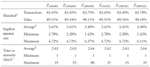
Note: Matched transactions and matched value correspond to the number of actual transactions and value of transactions (in percentage) that are identified by the algorithm, respectively. b Simple average. c Calendar days. d Instead of running the algorithm from the first to the last date, we run the algorithm backwards to mitigate the over-identification of long maturity transactions and examine the robustness of results. Source: authors' calculations
Table 3 exhibits how the algorithm for the selected scenario (Z (100|90)) solved for matches in transactional data. Single matches (i.e., only one refund is available as a plausible match) are the most common solution (94.45%). Multiple matches are uncommon (5.55% by number of transactions, 13.09% by transactions' total value), and most of them are solved by the first in first out rule (4.33% and 10.84%, respectively) -after the lowest time to maturity and the closest to the term structure rules have been exhausted. That is, for the selected dataset, the algorithm encounters multiple matches occasionally, and thus results are rather robust to the selection of solutions for multiple matches.
Table 3 Solving for single and multiple matches
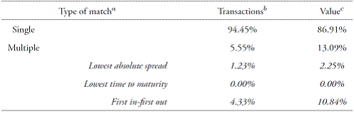
Note: a Based on the recursive procedure for solving multiple potential matches in Section II. b Calculated as the proportion of total loans in the sample. c Calculated as the proportion of total loans value in the sample. Single matches are the most common solution. Source: authors' calculations.
The graphical outcome of the algorithm for the selected scenario is displayed in Figure 2. Dots correspond to loans identified by the algorithm, whereas the line corresponds to our weighted average implicit interbank interest rate (IIR). All time to maturities available are displayed. The corridor corresponds to the selected scenario±100 basis points with respect to the maximum and mini-Z (100|90), and it is non-symmetrical due to its design (i.e., mum IBR for the overnight, one-month, and three-month time to maturities).
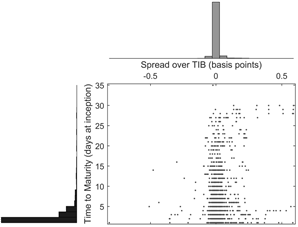
Other information valuable for monitoring purposes may be available as well. Figure 3 exhibits a scatter plot that relates identified loans cost and time to maturity; cost is expressed as a spread over the interbank overnight funds average rate (TIB), whereas time to maturity corresponds to the number of days at inception. Each axis displays a histogram that corresponds to how the cost and the maturity are distributed in the period under analysis. The average (median) spread over TIB is −0.0043 (−0.0090) basis points, with a minimum and maximum around 0.81 and 0.59, respectively. The average (median) maturity of interbank loans is about 2.6 (1) calendar days, with most deviations from the 1-day maturity corresponding to overnight loans coinciding with weekends or holidays. Altogether, Figure 3 depicts that most loans have a low time to maturity at inception (78.86% are overnight loans), and most loans spread over TIB tend to be rather small. As expected, there is a positive and non-negligible linear dependence between cost and time to maturity, with a correlation coefficient about 0.34; yet, correlation significantly diverging from unity reveals that -as expected- there is more to cost than time to maturity (e.g., credit risk, market liquidity).
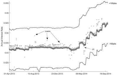
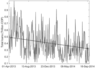
Figure 4 displays the total value of contracted loans for each day in the sample. A decreasing trend is noticeable. This is consistent with two changes in Central Bank's monetary stance depicted in Figure 1. First, in March 2013 the Central Bank halted a 12-month period of rate reductions. Second, in April 2014 the Central Bank began increasing its intervention rate. These two changes may explain to some extent the decreasing trend in interbank loans during the period under analysis.
B. Contrasting the selected scenario with reported data
Reports or surveys from financial institutions are the most common source of interbank data. Two types of reports are available from the Colombian Financial Superintendency, both containing different information reported by local financial institutions.
The first type is a report on the interbank funds transactions occurred during the previous business day. It is aggregated by lender, and reports the total value and weighted average interest rate of the loans for three maturities (i.e., overnight, 2-5 days, more than 5 days). After an exhaustive validation process, this report is used by the Central Bank to calculate the interbank overnight funds average rate (TIB). However, it does not contain information about the borrower; it is aggregated by maturity, and does not include the pending amount (i.e., the value of the claim). Hence, this type of report is useless for examining and monitoring individual loans and their financial conditions, or for calculating the exposures between financial institutions and building the corresponding interbank claims networks. Consequently, this type of report is discarded for the purpose of this article.
The second type of report discloses each outstanding interbank loan separately, reports the lender, borrower, and pending amount. Each outstanding interbank loan is identified by a unique code, which we use to determine the date in which the loan was contracted. Although the data has a daily frequency, it is made available to the Central Bank in batches transmitted with a lag of between one and two weeks.
As with most reports by financial institutions to financial authorities, the steps involved (i.e., consolidating, processing, transmitting) may result in lagged information and potential errors. Also, as contrasting the reported data is difficult and costly -if possible- for financial authorities, it is uncertain to what extent the information reported is reliable and complete. Furthermore, as the Colombian Financial Superintendency only requires credit institutions to report their interbank funds transactions, other financial institutions that are allowed to participate in the interbank funds market (e.g., brokerage firms) may not be considered.
In contrast, transactional data are available with a minimum lag (i.e., right after the market closes for overnight loans), and it may be monitored in realtime (i.e., as transactions are registered). As the algorithm requires the refunds to match the loans, there is at least a 1-day lag for the overnight loans. Unlike reports required by the Financial Superintendency, due to the non-tiered (i.e., direct) nature of the local large-value payment system, interbank funds transactions with or among non-credit institutions are captured and readily available.
Unfortunately, reliability and completeness of interbank funds transactional data in our case are uncertain as well. The quality of transactional data depends on how careful and truthful financial institutions are when using the codes assigned for registering transactions in the large-value payment system. As with reported data, it is difficult and costly -if possible- for financial authorities to verify that all interbank funds transactions are properly registered.
As the reliability and completeness of both data sources (i.e., transactional and reports) are uncertain, contrasting our results is not straightforward. We are trying to assess the quality of an algorithm run on a dataset whose quality cannot be verified by contrasting its results with financial institutions' reports whose quality has not been verified either. Thus, under the (unverifiable) assumption of reliability and completeness of financial institutions' raw reported data, we expect to find minor and reasonable differences when contrasting transactional data.
The contrast is as follows. We use the second type of report provided by the Colombian Financial Superintendency for the corresponding period (April 1, 2013-September 30, 2014). From this source of raw reported data, we build a consolidated and revised dataset containing the original loan and its main financial features (i.e., contracting date, lender, borrower, loan value, interest rate, and maturity).
Based on the consolidated and revised version of raw reported data we make four contrasts. First, we contrast the number and value of loan transactions identified from both sources; the less dissimilar the datasets, the less disparate the number and value of loan transactions. Second, we calculate the proportion of loan transactions identified from transactional data that coincide with those identified from reported data by date, lender, borrower, and loan value; the higher the proportion, the lower the occurrence of Type 1 errors (i.e., false positives). Third, we discriminate the interest rate matching precision of transactions coinciding from reported and transactional data; we discriminate between exact matches (i.e., zero two-decimal digit absolute difference) and approximate matches (i.e., absolute difference between 1 and 30 basis points). Fourth, we calculate the proportion of loan transactions from reported data that are also identified from transactional data by date, lender, borrower and loan value; the higher the proportion, the lower the occurrence of Type 2 errors (i.e., false negatives).
Table 4 presents the outcome of the contrast. The number and value of identified loans from each data source is rather dissimilar, with reported loans about 1.46 and 1.25 times that from transactional data, respectively. A reasonable explanation for such disparity is related to the loan-by-loan nature of reports required by the Financial Superintendency, even if the conditions (i.e., date, interest rate, maturity) could allow some aggregation. Also, as the large-value payment system charges a per-transaction fee,11 financial institutions may find optimal aggregating loans into a single registry, and may also aggregate refunds occurring in the same day. An alternative explanation may be the settlement of interbank loans and refunds outside the large-value payment system (e.g., by the delivery of cash or checks). Likewise, the separate settlement of the principal and interest may further complicate the identification of loans and their refunds; yet, the per-transaction fee charged by the large-value payment system should dissuade financial institutions from such separation. Therefore, such disparity may not be surprising, and should also increase the occurrence of Type 2 errors (i.e., false negatives).
The number and value of loans from transactional data that match reported data by date, lender, borrower, loan amount and interest rate is high, 99.70% and 99.83%, respectively; conversely, the number and value of loans from transactional data that do not match reported data is rather low, 0.30% and 0.17%, respectively. Exact interest rate matches (i.e., two-decimal digit precision) occur for 91.51% and 88.56% of the number and value of loans from transactional data, respectively. 8.19% and 11.27% correspond to approximate matches, which have an average absolute difference about 2 basis points. All in all, the proportion of loans from transactional data that match reported data suggests that Type 1 errors (i.e., false positives) are rare. Furthermore, as wrong matches can be considered a subset of false positive errors (Arciero et al., 2013), the low occurrence of Type 1 errors and the dominance of exact matches may be interpreted as a signal of a low occurrence of Type 3 errors (i.e., wrong matches).
Table 4 Contrasting transactional and reported data
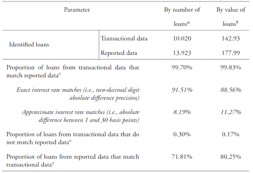
a Number of loans, unless otherwise stated. b Trillion $COP, unless otherwise stated. c A match is based on the exact coincidence of date, lender, borrower, and loan amount, whereas the interest rate match considers exact and approximate coincidences. Source: authors' calculations.
Concurrent with the number and value of loans from reported data exceeding those from transactional data, the proportion of loans from reported data that match transactional data is 71.81% and 80.25%, respectively. This suggests that Type 2 errors (i.e., false negatives) are non-negligible. A typical source of Type 2 error is a narrow corridor of plausible rates; however, Tables 1 and 2 show that widening the corridor does not increase the number or value of matched loans notably. Alternatively, as stated before, misusing large-value payment system's registration codes, the aggregation of loans in a single register in transactional data, the separate settlement of principal and interests, and the settlement of loans and refunds outside the large-value payment system may explain differences in the number and value of loans. Still, as the reliability and completeness of reported data is not verifiable, it is uncertain to what extent the excess of reported data and the occurrence of Type 2 errors are related to the quality of both reported and registered information.
C. Contrasting the implicit interbank interest rate with market data
As customary in the literature (see Millard & Polenghi, 2004; Heijmans et al., 2010; Arciero et al., 2013), we contrast our implicit interbank interest rate with the existing interbank interest rate benchmarks. In Colombia, there are two publicly available benchmarks: First, the interbank overnight funds average rate (Tasa Interbancaria - TIB), which is calculated and reported by the Central Bank based on financial institutions' reports to the Colombian Financial Superintendency. TIB is calculated after an exhaustive validation process of financial institutions' raw reported data, thus it is a reliable and comprehensive benchmark. Second, the interbank overnight reference rate (Índice Bancario de Referencia Overnight - IBRON ), which is the overnight rate of the interbank reference rate formation program. As IBRON results from the interest rate formation program, it is a reliable and comprehensive benchmark as well.
As both benchmarks are overnight rates, we build the corresponding implicit interbank overnight interest rate (IIRON ). That is, from the selected scenario (Z (100|90)) we discard all loans with maturities greater than one business day. Figure 5 displays IIRON, IBRON and TIB for the period under analysis (1 April, 2013-30 September, 2014). Due to the reliability and comprehensiveness of TIB and IBRON , divergences displayed by the implicit interbank overnight interest rate (IIRON ) should correspond to the features and limitations of our algorithm and datasets.
The similarity between the three interbank overnight interest rates is evident. Differences are scarce, and they are not prominent. Concurrent with loans cost distribution (see Figure 3), the implicit overnight loans (the dots) do not deviate too much from the three interest rates in the middle of the corridor.
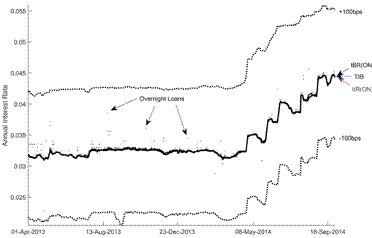
Table 5 confirms the linear dependence (i.e., correlation) among the three overnight interest rates level and serial differences, above and below the main diagonal, respectively. As in Heijmans et al. (2010), this correlation decreases the chance of Type 1 and Type 2 errors.
Table 5 Correlation of the three overnight interest ratesa
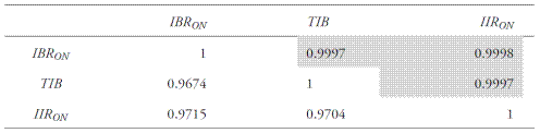
Note:a Correlation on the level (differences) is above (below) the main diagonal. Source: authors' calculations.
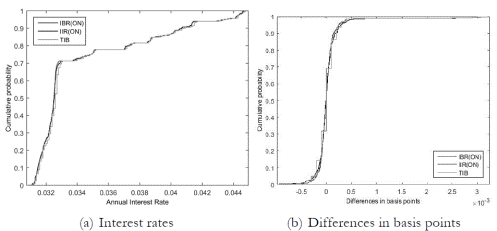
Likewise, Figure 6 confirms the correspondence of the cumulative distributions of interbank overnight interest rates and their differences. The two-sample Kolmogorov-Smirnoff test does not reject the null hypothesis that data in IBRON and IIRON are from the same continuous distribution at any typical significance level, either for interest rates (p-value =0.87) or their differences (p-value = 0.82). However, this test is rejected when the two samples are TIB and IBRON or TIB and IIRON .12
D. Interbank claims networks
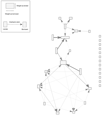
The algorithm does not only allow obtaining interbank interest rates from transactional data, or loans time to maturity and value. It also allows building the corresponding interbank claims networks in a straightforward manner.
The procedure added to the typical Furfine's method consists of organizing loans in matrix form, building a hypermatrix (i.e., a cube) of loans, with dimensions N ×N ×T. T corresponds to the number of days in the sample (t =1,2,...T), and N corresponds to the number of observed participants all over the sample (n = 1,2,...N). Each t-layer of the hypermatrix will accommodate the cumulated loans granted from financial institution i to financial institution j up to day t. Conversely, all refunds should be organized accordingly. Subtracting each layer in the refunds hypermatrix from the loans hypermatrix will yield the exposure (i.e., outstanding loan) hypermatrix, with each t-layer containing the interbank claims that i holds from j at day t (i.e., j has an outstanding loan from i at t). Hence, each resulting layer is the weighted adjacency matrix of interbank claims.
The graph corresponding to a randomly selected weighted adjacency matrix of interbank claims is portrayed in Figure 7. Nodes or vertexes (in rectangles) correspond to a financial institution that participated at some time t throughout the sample; for the period under analysis (1 April, 2013-30 September 2014), there are 31 participating financial institutions. The height (width) of each node corresponds to its contribution to the total claims of the market as a lender (borrower). The direction of the arrows (i.e., arcs) represents the existence of an interbank claim (i.e., from the lender to the borrower), whereas their width represents its contribution to the total claims of the system.
Final remarks
By implementing Furfine's method on a dataset from the Colombian large-value payment system this paper attained three main objectives. First, we filtered out interbank funds transactions in the Colombian market in order to identify interbank loans without relying on data reported by financial institutions. Results suggest that the algorithm is useful and robust as an alternative source of interbank loans data.
Second, we contrasted the loans identified by our algorithm with those identified from reports by financial institutions. Most loans identified by the algorithm coincide with reported data, and most of these coincidences are exact matches. Furthermore, the implicit overnight interest rates successfully match the publicly available overnight rates benchmarks. Such convergence of the implicit overnight interest rate is a fair test of the algorithm's goodness of fit. Interestingly, by running the algorithm backwards we mitigated the over-identification of long-term interbank loans in a straightforward manner.
Third, we constructed a hypermatrix containing the interbank claims network for each day in the sample from transactional data. As illustrated during and after the Great Financial Crisis, it is important to highlight that claims networks are vital for examining financial contagion and systemic risk (see Allen & Gale, 2000; Battiston, Delli et al., 2012; Battiston, Puliga et al., 2012; Kambhu, Weidman & Krishnan, 2007; Haldane, 2009; León & Berndsen,
2014).
Three main contributions from our results are worth highlighting. First, consistent with the lack of timely and granular information during the Great Financial Crisis, we provide further evidence on the usefulness of large-value payment systems' data for monitoring, overseeing, and analyzing the interbank funds market.
Second, we emphasize the importance of recent efforts by financial authorities to construct datasets in which unsecured transactions may be filtered out with ease. It is clear that efforts aiming at unusual datasets like ours or at collecting transaction-level data from financial institutions are advantageous. In this vein, as highlighted by Bank of England (2015), enhanced information on money markets benefits financial authorities' analysis of both monetary policy and financial stability.
Third, by running the algorithm backwards (i.e., starting with the last date of the sample until reaching the first one) we attained a practical method for mitigating the over-identification of long-term interbank loans, an issue also encountered by Guggenheim et al. (2010) and Heijmans et al. (2010). To the best of our knowledge, this backwards-run setup has not been attempted in related literature before, and may be worth exploring in further implementations of Furfine's algorithm.
Challenges arising from this methodological article come in several forms. First, attained numerical results allow for implementing financial contagion and systemic risk models, such as DebtRank (Battiston, Puliga, et al., 2012). Second, consolidating other sources of financial claims (e.g., derivatives, collateralized loans) into a multi-layer network may provide a broader view of financial contagion (see Poledna et al., 2015). Likewise, incorporating nonfinancial institutions (e.g., households, firms) into a multilayer network may provide a comprehensive view of systemic risk -as in De Castro and Tabak (2013). Finally, comprehensively tracking the dynamics of financial institutions' interbank loans (e.g., their cost, maturity, and counterparties), amid the dynamics of the interbank claims network (e.g., density, and distribution of links), may provide valuable information for authorities contributing to financial stability, and to formulating monetary policy.

