Introduction

The price elasticity of demand (PED) is one of the most important parameters in economic analysis and practical econometrics, as it gives the percentage change in the quantity demanded in response to a one percent change in price. Commodities such as oil and gasoline can be regarded as elastic in the short run (^{Lin & Prince, 2013}; ^{Neto, 2012}; ^{Arzaghi & Squalli, 2015}). These goods can be considered as produced and traded in competitive markets. Nevertheless, there are some commodities, such as electricity power, which pricing behavior does not follow the usual patterns described in the commodity pricing literature, so its PED could be more difficult to estimate. In the electric power industry, the study of demand elasticity serves to understand the reaction of consumers to price changes and the possibility that generators exercise market power (^{Labandeira, Labeaga & López-Otero, 2016}). Furthermore, the estimation of the PED in the electricity industry is important given the socio-economic impact that electricity has in contemporary society. Several factors have driven increasing interest in this issue in recent years. Such factors include the trend of electricity deregulation in several countries (^{Arango & Dyner, 2006}; ^{Pollitt, 2009}); new policies devised to mitigate the environmental impact of energy resource exploitation (MacCombie & Jefferson, 2016; ^{Nienhueser & Qiu, 2016}); and a growing concern for energy efficiency.

Demand estimation along with PED have been the focus of many studies. For example, industrial electricity demand studies are presented by ^{Kamerschen and Porter (2004}) and ^{Polemis (2007}) for USA and Greece, using simultaneous equations and cointegration methods, respectively.

^{Alter and Syed (2011}) used cointegration and vector error correction to determine the short- and long-run dynamics of electricity price and demand in Pakistan. ^{Beenstock, Goldin and Nabot (1999}) adopted dynamic regression and cointegration techniques to compute long-run elasticities in the household and industrial sectors of Israel, while ^{Bose and Shukla (1999}) estimated sectorial elasticities for small, medium and large firms employing a regression approach. ^{Agnolucci (2009}) estimated electric energy demand and price elasticity for German and British industrial sectors over the period 1978-2004 using disaggregated data. ^{Narayan and Smyth (2005}), ^{Halicioglu (2007}) and ^{Ziramba (2008}) used cointegration techniques to estimate the price elasticity of residential electricity demand in Australia, Turkey and South Africa, respectively; while ^{Alberini and Fillippini (2011}) applied partial adjustment models to estimate the price elasticity of household electricity demand in the USA.

^{Lijesen (2007}) presented a study on real-time price elasticity of electricity demand in the Netherlands. He provides a quantification of the real-time relationship between total peak demand and spot market prices, finding a low value of the real-time price elasticity, which might be explained by the fact that not all consumers observe spot market prices. In Thimmapuram et al. (2010) and Thimmapuram and Kim (2013), the modeling and simulation of the price elasticity of demand in Korea was carried out using a representative agent-based model within a smart-grid environment. It is shown that being well equipped with smart grid technologies increases a consumer’s awareness of responsiveness of demand. Also, a price-elastic consumer benefits from a reduction in electricity usage and prices and contributes to reduce congestion as well as market power.

^{Bernstein and Madlener (2015}) estimated electricity demand elasticities for different subsectors of the German Manufacturing Industry from 1970 to 2007; employing a cointegrated VAR approach and taking into account structural breaks, they found long-run relationships among sectors and estimated short-run elasticities using a single-equation error correction modeling. Oka- jima and ^{Okajima (2013}) estimated the price elasticities of residential demand in Japan from 1990 to 2007. They found that the price elasticity of residential electricity demand in Japan is highly affected by income inequality and severe weather. Bernstein and Griffin (2006) estimated regional differences in price elasticity in the US, finding that demand was relatively inelastic to price, and that this relationship had not changed significantly between 1977 and 1999. Other studies regarding the estimation of elasticity of residential demand are presented in ^{Athukorala and Wilson (2010}) and ^{Arthur, Bond and Wilson (2012}) for Sri Lanka and Mozambique, respectively.

^{Labandeira et al. (2012}) use real data on prices and electricity consumption from Spain to present a model of incomplete information and in which households and large consumers are taken into account to estimate the price elasticity of electricity demand. The authors found that electricity demand is inelastic with respect to its price in the short term, although there are differences between residential and industrial demand. In the case of households, demand elasticity diminishes as the level of per-capita income increases; however, this relationship was not found in the case of large companies.

^{Cárdenas, Vásquez and Whittington (2014}) performed a study regarding price elasticity of the demand for electricity, oil and gas in Chile. They found that, among these goods, electricity is the most inelastic, with values ranging between -0.10 and -0.60 for the three main manufacturing sectors. ^{Labandeira et al. (2016}) carried out a meta-regression analysis that intends to adjust the price elasticities of electricity demand, identifying the main factors explaining the differences between the results of the selected studies, such as country, type of consumers, data, models, sample period and estimation methods.

In this paper, we are interested in estimating the PED of electricity forward contracts in the manufacturing industry of Colombia. To this end, we performed multivariate analysis. Initially, we used a vector autoregression (VAR); however, due to its poor performance in terms of the impulse response function (IRF), we used a structural vector autoregression (SVAR) to estimate the elasticity of demand and to simulate the response of demand to an impulse in the electricity price. The econometric analysis is based on monthly observations of historical time series between 2005 and 2012, considering economic activities (disaggregated up to two-digit International Standard Industrial Classification codes) at different voltage levels. Our focus is on five electro-intensive sectors: food and drinks, plastic and rubber, retail trade, textile manufacturing and chemical industry.

After an exhaustive survey of the existing literature on estimation of the PED in Colombia, we found out that this type of estimation has been rarely done. To the best of our knowledge, this is the first paper that employs the VAR and SVAR approaches to estimate the PED in Colombia. The contribution of our paper can be summarized as follows: first, it adds to the small body of empirical literature on this matter in Colombia; second, it specifies the relationship of industrial electricity demand as a function of electricity prices, industrial production index, and hydrology; third, it provides consistent estimations of the PED; and, finally, it computes (when possible) the IRF.

This paper is divided as follows. In section I, we describe Colombia’s electricity market and report some studies related to its electricity demand and PED. In section II, we introduce in a straightforward manner the VAR and SVAR methodologies and describe the empirical strategy adopted for estimating PED. In section III, we present and analyze our results. We conclude with a summary of the main conclusions.

I. The electricity market in Colombia

The electricity market in Colombia is composed of two main markets: a spot market and a bilateral market based on non-standardized contracts. An independent system operator (ISO) solves the ideal dispatch in the spot market. Rather than minimizing the hourly costs of generation, the objective function of the ISO is to set an economic dispatch (twenty-four hour optimization problem), where generators submit bids and side payments are introduced. The bids specify electricity offer prices for the next twenty-four hours, startup costs and maximum generating capacity for each hour in the next day. Once the optimization problem of the ideal dispatch is solved for the twenty-four hours, the equilibrium price is calculated as the price bid of the marginal plant that is not saturated. The hourly spot price is defined as the equilibrium price plus an uplift (^{De Castro et al., 2014}).

Also, Colombia’s electricity market works on a 24-hour-ahead pool through which all electricity is dispatched, regardless of any short-, medium- or long- term bilateral agreements between agents. These agreements are materialized in bilateral contracts called forward contracts. It is a stylized fact that electricity demand in this market does not change (or it does at a too slowly pace), and this is especially evident in the spot market. Actually, the demand is a constant (a given fact) for setting the spot price, and, on the other hand, the market supply is built based on the daily-bid prices and the hourly-declared availability of the power generators. Therefore, in the electricity market of Colombia, the fundamental factors of short-term electricity pricing are hydrology as well as the incentives and expectations of the agents and their strategies in the spot market. However, electricity pricing in the forward contract markets is very different, and therefore the analysis of demand behavior and its response to changes in prices is harder to investigate. While in the spot market there is perfect information about prices, forward contracts constitute private information for agents, so many variables are not directly observable. The only available information consists of averages of prices and quantities demanded of energy in contracts. It is worth to mention that every forward contract is very different in time and procedures. This paper focuses on the estimation of the PED for the electric power industry in such forward contract markets in Colombia.

A forward contract is a financial instrument; more precisely, it is a power purchase agreement, which aims to protect agents from the risk to buy and sell at the spot market. In Colombia’s electricity market, there are two typical agreements: consumption-based payment contract and Take or Pay contract. Their duration and price depends on the needs and bargaining power of agents. In general, agents behave strategically and the choice to buy and sell energy in forward contracts or in spot markets is based on their private information and the volatility of spot prices. This is because in both markets, even as they are trading exactly the same good, prices are dramatically different. This is one of the most criticized features of bilateral contract markets, because it makes the market very inefficient. In fact, any relationship between contract market price and hydrology vanishes, while that does not happen in the spot market.

Few studies and analysis regarding electricity demand and the PED in Colombia’s electricity market have been found. An exhaustive search in bibliographic databases produced a few related papers that date back to the early 1990s. For instance, ^{Botero, Castaño and Vélez (1990}) studied industrial electricity demand in Colombia in the period 1970-1983. After not rejecting the hypothesis of complementarity between electrical energy and the capital stock, they carried out a parametric estimation of demand in terms of the capital stock. According to these authors, the rational business decision of the firm is not to use electricity as input, as this is a direct consequence of the existence of capital and the technical requirements inherent to the assumed production function. In fact, the decision problem of the firm is whether to buy power from the grid or to be self-generating because the empirical evidence suggests the existence of a substitution effect between these two alternatives in the long run.

^{Ramírez (1991}) developed a model in which the demand for electricity in Colombia’s industrial sector is explained by the capital stock, the labor factor and energy considerations. He splits the data into two groups: high and low electricity consumption sectors. His results suggest that in the sector of high electricity consumption, demand for electricity depends primarily on non-energy factors; while in the low consumption sector, demand for electricity depends on the conditions of energy as an input. These results confirm the existence of complementarities between electricity and capital and substitutability between energy and labor due to the intensive and extensive use of capital in the first group (large companies) and the intensive use of labor in the latter.

^{Barrientos, Olaya and González (2007}) presented a non-linear spline model for demand estimation in the electricity market of Colombia. They modeled the daily electricity demand in the southeast region of the country through the implementation of a non-parametric regression model. They considered some calendar variables such as time of the day, day of the week, month, and year, among others, in the estimation process. ^{Maddock and Castaño (1991}) and Maddock, Castaño and Vella (1992) carried out estimates of residential electricity demand in Medellin (Colombia), where prices follow a rising block scheme. They concluded that the price elasticity of demand is greater in the well-off residential areas of the city. ^{Franco, Velásquez and Olaya (2008}) characterized monthly electric power demand in Colombia using a model of non- observable components from 1995 to 2006. They found that the monthly growth in demand has a linear deterministic component, approximately constant in recent years. Finally, ^{Espinosa, Vaca and Ávila (2013}) used an autoregressive distributed lag model to estimate price elasticities of residential and industrial demand in Colombia, finding that residential demand is more inelastic than industrial demand.

II. Conceptual framework and methods

Multivariate time series analysis is an instrument for modeling variables that are correlated in time, unlike univariate models which do not allow such an analysis. However, the ability to take multiple time series to be included in a single model has drawbacks to be analyzed prior to use. For example, it is necessary to determine whether the various time series satisfy the covariance stationarity conditions, which are very important features for allowing identification of the type of multivariate structure that has to be implemented.

If preliminary analysis of data indicates that the process is covariance- stationary (that is, the mean, variance and auto-covariance do not depend on the time in which the sample was taken), the typical procedure indicates that it is possible to use vector processes without restrictions on data, the most common of which are VAR models. However, if the process is not stationary, the suggested procedure consists of looking for long-run relations between some (or all) of the variables, which necessarily leads to the notion of cointegration.¹

Finally, it is important to highlight that VAR models also support the inclusion of exogenous variables as explanatory variables, but in this case it is not possible to compute either the impulse-response function or the variance decomposition. The inclusion of explanatory variables in the VAR just allows one to compute the marginal effect on the endogenous variables.

A. Empirical Specification

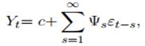
In general, a VAR model can be written as:

(1)

where is an n X 1 vector for all t, εt is a white noise disturbance term, therefore Φј is a matrix of dimension n X n for j = 1, 2, . . . , p. Note that the inclusion of more variables and more lags could make the estimators very inefficient in terms of significance of the parameters. Moreover, if the number of parameters exceeds the number of observations, then the identification conditions are not satisfied and it is not be possible to carry out the estimations (^{Hamilton, 1994}).

The implicit assumptions of the VAR can be summarized as follows: first, for a covariance stationary process, matrices Φj, j = 1, . . . , p, in (1) can be defined as the coefficients in the projection of Yt on p lags of Yt, so εt is not correlated with Yt j, j = 1, . . . , p, by the definition of Φ1, Φ2, . . . ,Φp. The parameters of the VAR can be consistently estimated by ordinary least squares by performing n independent regressions. Second, the assumption that Yt follows a pth-order VAR process is basically that p lags are sufficient to summarize all the dynamic correlations among elements of Yt. Under the stationarity assumption of every series in Yt, model (1) can be written as:

(2)

which is a vector autoregressive moving average process where Ψ _s is a n X n matrix interpreted as the impulse-response function (IRF). It is easy to check that

(3)

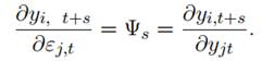
Thus, equation (3) admits the following interpretation: the element (i, j) of matrix Ψ _s identifies the consequences of an increase of a unit or one standard deviation n the innovations ^_εj at time t on the values of the variable yi in t + s, holding constant the innovations in other times. It means that

(4)

Assuming that ^_yit represents the electricity demand at time t and ^_yjt represents its price, once the VAR is estimated we can compute the IRF and evaluate the effect of a shock on prices on the demand for s = 1, 2, 3, . . . periods ahead. More specifically,

(5)

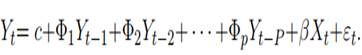
The effect of the electricity price on electricity demand given by expression (5) represents the dynamic PED. As we noted above, the VAR also sup- ports inclusion of exogenous variables. Let X be a T ×k matrix of exogenous variables, such as hydrology (water input in kWh) or the industrial production index (IPI), then the VAR(p) can be expressed as:

(6)

Being X an exogenous matrix, then the parameter β only indicates the impact of the exogenous variables on endogenous ones; however, it is not possible to compute the impulse-response functions. Moreover, the underlying vector moving average representations of equation (6) is given by

(7)

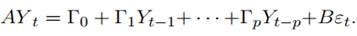
where ^_Ds are the dynamic multipliers and Ψ _s has the same IRF interpretation as in equation (2). Eventually, we could be interested in estimating a special type of vectorial process known as structural VAR, denoted by SVAR(p). It is easy to check that VAR (equation 6) can be deduced from the SVAR, which has the following specification:

(8)

As with VAR, it is possible to calculate the impulse-response function associated with SVAR, with the same interpretation for the elasticities. The fundamental difference between a VAR and a SVAR is that the latter identifies the structural shocks. Parameters in matrices are called structural coefficients; parameters in matrix A show the contemporaneous effect of one specific set of variables on the other set of variables of interest. Moreover, it is possible, for example, to impose restrictions on the parameters in matrix A to calculate the effect of one variable on another specific variable, but not on the others, so these parameters can be interpreted as the PDE.

In general, the structure of SVAR models is given by equation (8), where matrix B is usually taken as the identity matrix. This specification is called the AB model, where the identification restrictions are imposed according to the underlying economic problem. The model estimation is performed in two steps. First, the model is estimated in reduced form (standard VAR):

(9)

where ^_Aj = ^{_A− 1}Γ _j for j = 1, . . . , p and ^_ut = ^{_A− 1 _Bεt} are the residuals. The second step is to estimate the matrix A of the SVAR model (for maximum likelihood) in consideration of the fact that an estimate of errors is obtained from the first step. This estimate of errors is given by uˆ _t = ^{_A− 1 _εt} or Auˆ _t = ^_εt . The impulse response function associated with the SVAR can also be calculated from these estimated innovations.

B. Data

The database used in this study focuses on price and demand for electricity forward contracts, by branches of economic activity and by voltage level. Five branches of economic activity were selected: food and drink sector, textile manufacturing, chemical industry, plastic and rubber manufacturing and retail trade sector.

The data source was XM, the company that operates the national interconnected system and runs Colombia’s electricity market.² Since the data are compiled on a calendar daily basis, we obtain monthly data by taking weighted averages of prices according to the size of demand for every branch of economic activity. Data set of price and demand starts in June 2005 and ends in September 2012, so we got 88 monthly observations.

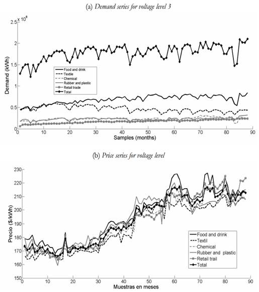
As usual, in every branch of economic activity, electricity consumption increases and price decreases with the voltage level, except for the retail trade sector where the electricity demand at voltage-level three is lower than that at

other voltage levels. However, the trend is that prices keep decreasing as the voltage level gets higher. The behavior of price and demand described in Table 1 is typical of Colombia’s electricity market if we take into account that the observed price comes from bargaining on forward contracts, which include negotiation of high electricity volumes. Figures 1 to 3 show the evolution of demand and price by voltage level.

Table 1 Descriptive Statistics 

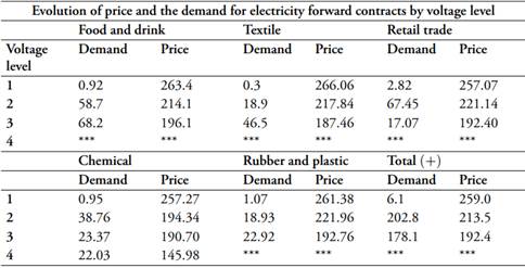
Note: *** Time series not available. (+) Total corresponds to the average of the price and the sum of electricity demand for the five industrial sectors. Demand measured in GWh. Price in COP/kWh.

Source: own calculations based on XM data.

Source: own calculations

Figure 1 

Source: own calculations

Figure 2 

Source: own calculations

Figure 3 

III. Empirical results

A. Stationarity Analysis

In order to stablish the stationarity of the data generating process, we perform an augmented Dickey-Fuller test and a Phillips-Perron test as shown in Maddala and Kim (1988). Table 2 shows the results of the testing procedure for each series in every voltage level.

Table 2 Phillips-Perron test 

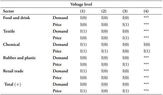
Table 2 shows t Note: ***Time series not available. (+) Total corresponds to the average of price and electricity demand in the five industrial sectors.

Source: own calculations based on XM data.

Table 2 show that in some cases the null hypothesis of a random walk process could not be rejected. In these cases, we applied the (1 L) operator in order to estimate the VAR/SVAR. For instance, series of demand and price for the chemical sector at voltage level 1 and price series for the food and drink sector at voltage level 3 have a unit root. It is worth noticing that we cannot find evidence of a long-run relationship (or co-integrated vectors) between

the variables. For this, we used the well known methodology developed by ^{Engle and Granger (1987}). Statistics tests do not allow us to reject the null hypothesis of a unit root, so we cannot perform vector correction models (VEC); instead, we use VAR models.

B. Standard VAR and the impulse-response function

We estimate VAR models for every branch of economic activity and every voltage level. In each case, we include price and demand in the forward contract as endogenous variables. Also, we add in a constant, the industrial production index and hydrology as exogenous variables. Figures 4 and 5 show the monthly trends of hydrology and IPI, two typical exogenous variables in the period under consideration. The data source for hydrology and IPI is XM and National Department of Statitsics (which stands in Spanish for Departamento Nacional de Estadística or DANE) respectively. It is worth to mention that the residuals produced by all models are stationary processes.

Source: own development based on XM data

Figure 4 Evolution of monthly hydrology 

Source: own development based on DANE data

Figure 5 Evolution of the industrial production index 

The lag-length testing is carried out by performing a likelihood ratio (or LR) test. Results suggest that the optimal lag number to be included in the VAR is between 10 and 12. Thus, we included 12 lags in each regression because we had monthly data. In doing so, we explored and took advantage of all the information contained in the dynamic relationship between demand and price.

As we mentioned above, rigorously speaking, the PED in dynamic and vector models is estimated through the impulse-response function. The IRF simulates the effect of a rise of 1% in the electricity price on electricity demand 12 months ahead. However, our simulations yielded that the IRF is not statistically significant (see figure 6).

The following graphs illustrate our empirical results, showing the lack of significance of the estimated IRF (solid line) since the upper band is entirely above zero and the lower band is below. Similar results are obtained when the auto-regressive vectors are estimated by branch of economic activity. In many cases, statistically significant lags of prices are obtained; however, the IRF estimate is not significant.

Source: own calculations.

Figure 6 Impulse-response functions 

The statistical exercises show that there is not a strong relationship between price and demand in the forward market. This means that long-term elasticities are not detected using the methodology of impulse-response functions. Furthermore, the results obtained suggest that the collected data does not have the best quality to model the relationship between demand and price of long-term contracts. In particular, the way in which the prices of contracts and the quantities demanded are reported to the market operator makes it difficult to identify the data generating process.

C. Structural VAR: short-run approach

We compute IRFs for the SVAR model; however, it yielded disappointing results in terms of statistical significance of the underlying parameters. So, given the discouraging results using IRFs by performing reduced VAR as well as SVAR, structural parameters are estimated having as reference the specification of the model given by (8). We use as endogenous variables the prices/rates and sales/demand by branch of economic activity, and, as exogenous variables, again hydrology and IPI are used. The restrictions imposed on each model are given by the matrix

(10)

which explicitly indicates that we are interested in the effect of a change in price on the demand for electricity. Note that an estimate of the parameter ϕ ₁₂ with positive sign is interpreted as a negative effect of price on the demand for electricity (see equation 8). Table 3 shows the contemporaneous (short-term) elasticities estimated in each model. The critical value of the normal distribution is in parentheses. It should be around 1.96 or higher to be considered significant at 5% or less. As in the case of reduced VAR, the residuals from SVAR are also stationary processes.

The estimated structural parameters show the change in demand for a positive variation in contemporary price of 1%. Note that for voltage level 1, the estimated parameters are significant and with the expected sign (negative) for all branches of economic activity, except for the chemical and textile sectors. In voltage level 2, the results are consistent and, except for the textile sector, all branches of economic activity show a reduction in demand when the price level increases by 1%. The same happens with voltage level 3, except for chemicals. The only sector with an elastic demand is food and beverages in voltage level 2.

Table 3 Estimated structural parameters 

Note: t values in parenthesis.

Source: own calculations.

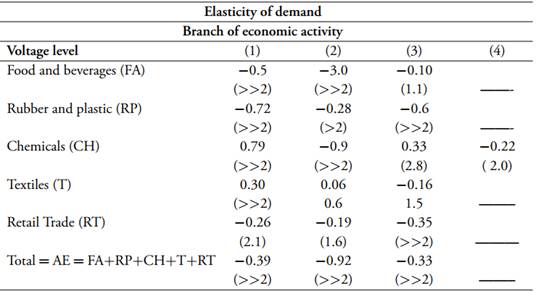
However, we find that the low response of the quantity demanded, considering a marginal change in price, shows that it would be convenient to make a seasonal adjustment of forward prices (or in the way in which the information is broadcasted).

Conclusions

In this paper, we estimated the PED of forward contracts in the electricity market of Colombia considering several economic activities at different voltage levels. The study of demand elasticity is important not only to discuss the possibility of this market to operate competitively, but also because nowadays there is a technical debate around the possibility of designing seasonal forward contracts in Colombia. Estimating the PED provides valuable information to market agents in order to construct complete contractual arrangements, especially in the presence of asymmetric information.

In order to compute the PED we described why an SVAR model, and their associated matrices, constitutes an appropriated framework for its estimation. Our main result suggests that some sectors, like food and drink or plastic and rubber manufacturing or even the retail trade sector, are slightly more sensitive to shocks on prices than the chemical industry or the textile sector. The only economic sector that displays a more elastic demand is food and drink manufacturing in voltage level 2. However, our general conclusion is that the industrial sectors analyzed show that electricity demand in forward contracts is almost inelastic to price variations. This result is consistent with what we would expect in an oligopolistic market such as the Colombian one.

The implication of these general results is evident: traders have lots of degrees of freedom for manipulating contract prices; then, this failure in functionality of contract markets gives traders a sort of market power. There- fore, forward contracts in the electricity market of Colombia are in need for changes, making all information about prices and quantities demanded public for all agents. This opens the possibility of investigating and implementing seasonal forward contracts, which may complement the spot market making Colombia’s electricity market more competitive