English (pdf)
 Article in xml format
 Article references
 Send this article by e-mail
 Cited by SciELO
  Cited by Google
  Similars in
SciELO
Similars in
SciELO  Similars in Google
 Permalink
Introduction
This study aims to examine dynamic interactions between wealth accumulation, gold distribution between monetary and non-monetary uses, and government policy under the gold standard. As far as the growth mechanism is concerned, the model of this study is developed within the framework of the neoclassical growth theory. The seminal paper in this field is due to Solow (1956). The theory is mainly concerned with endogenous physical capital or wealth accumulation (Burmeister & Dobell, 1970; Azariadis, 1993; Barro & Sala-i-Martin, 1995). We follow the Solow model in modeling economic production. We analyze household behavior using the approach proposed by Zhang (1993) and introduce gold based on Barro’s (1979) approach.
Furthermore, this study aims to examine gold price dynamics within a neoclassical growth model under the gold standard. Dynamics of gold prices are well mentioned but not properly theoretically examined within a modern growth theory with endogenous wealth accumulation. There are many empirical studies on gold prices and the real rate of return on gold (Dubey, Geanakoplos & Shubik, 2003; Ranson, 2005; Dempster, 2009; and Seemuang & Rompreert, 2013). Forces of supply and demand for gold are not like other commodities. On the supply side, the amount of gold stock changes very slowly. On the demand side, most of gold is used for jewelry, coin collections and central banks, with less than 10% used for industrial production (Thomas, 2015). This study follows some dynamic models on gold prices (Barro, 1979; Bordo & Ellson, 1985; Dowd & Sampson, 1993; Chappell & Dowd, 1997). We deviate from previous studies mainly in that our model also takes account of both wealth accumulation and physical capital accumulation, something neglected in most of the preceding literature. As saving can be conducted by keeping gold and accumulating wealth, dynamics of gold prices should be closely related to physical capital accumulation and other variables. We study the dynamic interdependence between economic growth and gold prices. It should be noted that although the gold standard has been abandoned a century ago in terms of its use as a medium of exchange and the monetary use of gold is quite limited even since the end of World War I, our study is theoretically meaningful as it provides insights into possible relations between gold values and economic variables.
Many of the most intriguing and important questions in dynamic economic analysis involve money. It is generally agreed that modern analysis on the dynamic interaction between inflation and capital formation begins with Tobin’s seminal contribution in 1965. Tobin (1965) deals with an isolated economy in which “outside money” competes with real capital in the portfolios of agents within the framework of the Solow model. In our approach, the money supply is based on Barro (1979), who pointed out that “It is frequently argued that the deflationist tendency of the gold standard can be countered by supplementing the world's gold stock with some form of paper gold. For example, the plans suggested by Keynes (1943), Triffin (1960, part II), and Mundell (1971, pp. I35-6) can be viewed in this context.” (p. 21). This study introduces paper money under the gold standard into the neoclassical growth theory. Rather than assuming some demand function for money like in Barro’s approach, we derive money demand from the optimal decision of households. We apply the money in the utility (MIU) function approach. This approach was used initially by Patinkin (1965) and Sidrauski (1967). In this approach, money is held because it yields some services and the way to model it is to enter real balances directly into the utility function (Zhang, 2009).
This study proceeds as follows. Section I introduces the basic model. Section II simulates it. Section III carries out comparative dynamic analyses regarding some parameters. The last section concludes.
I. The basic model
The model is built upon a few approaches in the literature on the theory of economic growth. In particular, the production sector is based on the Solow model, the gold standard and price dynamics are based on Barro (1979), and household behavior is based on Zhang (1993, 2009). The money demand in Zhang’s approach is based on the traditional MIU model (Sidrauski, 1967). As in the Solow growth model, the economy has one sector producing a single commodity for consumption and investment. Capital depreciates at a constant exponential rate, ( k , which is independent of the manner of use. The technology of the production sector is characterized by constant returns to scale. All markets are perfectly competitive. Factors are inelastically supplied and the available factors are fully utilized at every moment. Saving is undertaken only by households. All earnings of firms are distributed in the form of payments to factors of production. Households own assets in the form of physical wealth and gold. They allocate their incomes to consumption and wealth accumulation. Population is homogeneous. Let N stand for the fixed population.
A. The production sector
The production sector uses capital and labor as inputs. Let K(t) stand for the capital stock at time t. We use F(t) to represent the output level. The production function is
 (1)
(1)
where A, ( and β are parameters. Markets are competitive; thus, labor and capital earn their marginal products, and firms earn zero profits. Let the rate of interest and the wage rate per unit of time be denoted, respectively, r(t) and w(t). For any individual firm, and are given at any point in time. The production sector chooses and to maximize profits. The optimality conditions are
 (2)
(2)
where p(t) is the price of the commodity.
B. Money supply
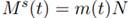
Following Barro (1979), we now describe the money supply. Let M(t) stand for the stock of money at time t. This stock is denominated in a nominal unit such as yen. This stock represents the liabilities of the central bank. Money takes the physical form of paper claims. As in Ricardo (1821), it is assumed that the bank is ready to buy or sell any amount of gold in exchange for money at the fixed (yen) price p G (t). Let G b (t) denote the stock of gold held by the central bank. As in Barro, total money supply is
 (3)
(3)
where the parameter ( measures the gold backing of the monetary issuance.
C. Households’ choice between physical wealth and gold
This study assumes that money is used only by households.1 The demand for money per household is denoted by m(t). Aggregate demand for money is
 (4)
(4)
Gold can be sold and bought in free markets without any frictions and transaction costs. Gold use will not waste. Households can own money, gold and physical wealth. In order to model the cost of keeping and using gold, we assume that gold can be “rented” through markets for decoration. We consider that the gold that is owned by the representative household can be used either by the household for decoration or rented out to other households. The rent of gold is denoted by R G (t). Consider now an investor with one unit of money. He can either invest in the capital good, thereby earning a profit equal to the net own-rate of return r(t)/p(t), or invest in gold, thereby earning a profit equal to the net own-rate of return R G (t)/p G (t). We assume that capital and gold markets are in competitive equilibrium at any point in time, so the two options must yield equal returns, i.e.,
 (5)
(5)
This equation enables us to determine the choice between owning gold and physical wealth. Daily life experience tells us that this assumption is made under many strict conditions. For instance, we neglect any transaction costs and any time needed for buying and selling goods. Equation (5) also implies perfect information.
D. Behavior of consumers
Unlike the optimal growth theory, in which utility defined over future consumption streams is used, we do not explicitly specify how consumers discount future utility resulting from consuming goods and services. This study uses the approach to consumers’ behavior proposed by Zhang (1993). Extensive explanations and many examples applying this approach are provided by Zhang (2005, 2006). Let ((t) and  , respectively, stand for the inflation rate and the per capita (physical) wealth. We have
 (6)
(6)
Let  stand for the amount of gold owned by the representative household. Current income per capita is given by
 (7)
(7)
where  is the interest payment,
  is the rent revenue from owning gold, w is the wage payment, and (m is the cost of holding money. Let a(t) stand for the total value of assets that the representative household owns. We have
 (8)
(8)
The total value of wealth that the representative household can sell to purchase goods and to save is equal to a(t). Here, we assume that selling and buying wealth can be conducted instantaneously without any transaction cost. Disposable income is the sum of current income and total value
 (9)
(9)
At each point in time, the household distributes the total available budget between money balances, m(t) the amount of gold for decoration/ornament,  saving, s(t) and consumption of goods, c(t). The budget constraint is given by
 (10)
(10)
From (10), (8) and (9), we have
 (11)
(11)
where

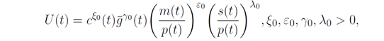
In Zhang’s approach, the utility function is dependent on saving from disposable income, consumption, gold holdings, and money holdings (Zhang, 2006). In this model, the representative household has four variables to decide on: s(t), c(t), m(t), and  .The consumer’s utility function is specified as follows:
 (12)
(12)
in which (0, (0, (0, and (0 are the elasticities of utility with respect to industrial goods, gold, real money holdings, and real savings. We call (0, (0, (0, and (0 propensities to consume industrial goods, to use gold, to hold real money, and to save, respectively. Maximizing (12) subject to (11) yields
 (13)
(13)
where

E. Closing the model
1. Wealth accumulation
According to the definitions of s(t) the change in the representative household total wealth is given by
 (14)
(14)
This equation simply states that the change in wealth is equal to saving minus dissaving.
2. Gold market clearing
The amount of gold owned by the population is equal to the amount of gold used by the population
 (15)
(15)
5. Physical capital accumulation
The accumulation of physical capital is described by
 (18)
(18)
This is simply an accounting relation.
6. Physical capital market clearing
The total physical capital is owned by the households
 (19)
(19)
We have thus built the dynamic model. It should be noted that the model is general in the sense that the Solow model can be considered as a special case of our model. Moreover, as our model is based on some well-known mathematical models and includes some features that no other single theoretical model explains, we should be able to explain some interactions that other formal models fail to explain. We now examine the dynamics of the model.
II. The dynamics and its properties
The economic system contains many variables. These variables are nonlinearly related. For illustration, the rest of the study simulates the model. In order to simulate the model computationally, we provide a programming procedure so that anyone can easily follow the motion of the economic system with any set of parameters and initial conditions. In the Appendix, we show that the dynamics of the economy can be expressed by three differential equations.
Lemma: The dynamics of the economy is governed by the following three-dimensional system of differential equations:
 (20)
(20)
where  and are functions of
and .
and are functions of
and .
Proof: see the Appendix.
Moreover, all the other variables are determined as functions of
and by the following procedure: and by (A2) → by (A7) → by (A14) → by (A12) → by (A10) →  by (A5) →
  , and by (13) → by (19) → by (1) →
 →
→  →
→  by (A3).
The system of differential equations (20) has three variables: 
 and
and  As shown in the Appendix, the expressions are complicated, so it is difficult to explicitly derive economic implications from the three equations. For illustration, we simulate the model to illustrate the behavior of the system. In the remainder of this study, we specify the parameters in Table 1 as follows:
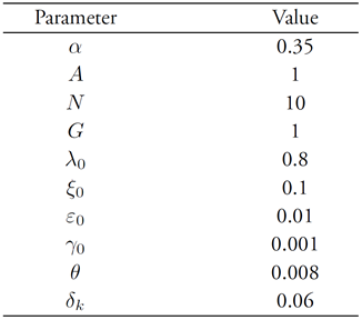
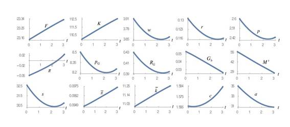
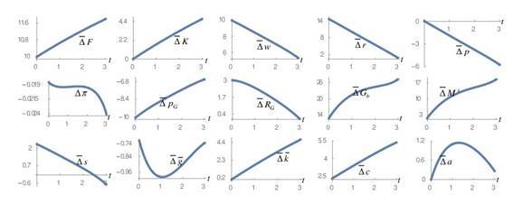
The propensity to save is 0.8 and the propensity to consume is 0.1. As the propensity to save implies that the proportion of disposable income used for saving and disposable income is the sum of the value of wealth and current income. The assumed value of (0 simply implies that 80 percent of household disposable income is for saving. Total factor productivity is A = 1. The amount of gold is 1 and the population is 10. The propensity to hold money is 0.01 and the propensity to use gold is 0.001. In regard to the preference parameters, what are important in our study are their relative values. The gold backing ratio is 0.008. The depreciation rate of physical capital is 0.05. To follow the motion of the system, we specify the initial conditions 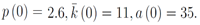
The simulation results are plotted in Figure 1. We simulate the model in a short period of time. The reason is that the system is unstable, as explained later. It does not have a stable equilibrium point. Due to the initial conditions, total output and the capital stock are increased. As the wage rates fall, both men and women work longer hours. Their leisure hours are reduced. The economy’s wealth and output are increased in association with rising labor force. Nevertheless, both consumption level and wealth per household are reduced.
We calculate the three eigenvalues: 
As two of the three eigenvalues’ real parts are positive, the equilibrium point is unstable. Thus, the system tends to be away from its equilibrium point if it is not located at it.2 If the system is unstable, comparative static analysis provides little insight into its behavior. In our model, long-run price stability is not guaranteed.3 If a system is not stable, it is hard to predict the long-term consequences of any change in the parameters. As our model explicitly shows the dynamic path of the economic system, we can conduct comparative dynamic analysis effectively at least during a short period of time.
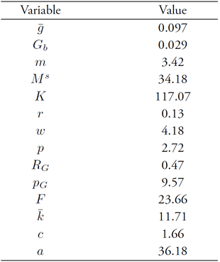
The simulation confirms that the system has the following equilibrium point. We list the equilibrium values of the variables in Table 2 as follows:
III. Comparative dynamic analysis through simulations
We simulated the motion of the economy under (21). We now examine how the economic system reacts to some exogenous change. As the lemma gives the computational procedure to calibrate the motion of all the variables, it is straightforward to examine the effects of a change in any parameter on transitory processes as well stationary states of all the variables. It should be noted that we do not describe the changes in the equilibrium point, as the system is unstable, and it provides little information about the motion of the dynamic system in the long term. Let  stand for the percentage rate of change of the variable
  due to changes in the parameter value.
A. A rise in the gold backing ratio
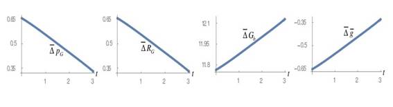
As in Barro (1979), we consider that a reduction in paper gold can be modelled by a rise in ( . We specify the increase as follows: 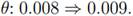 This implies that the money stock is reduced for a fixed amount of gold backing. The simulation results are plotted in Figure 2. The variables whose values are not affected by the parameter change are not included in Figure 2. The gold price and gold-use cost fall during the period of simulation. The government holds more gold and the household holds less. As in Barro (1979), a change in ( has no effect on the equilibrium values of the price level and money stock. In our approach, changes in ( only affect the gold distribution, gold price and gold-use cost. The reason for this difference is that we take account of households’ gold holding.
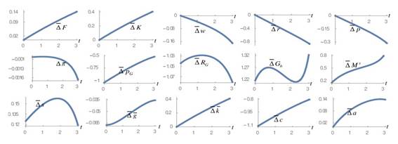
B. Fall in the propensity to hold paper money
We are now concerned with how the propensity to hold paper money affects economic growth. We reduce the propensity to hold paper money as follows: 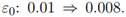 The simulation results are plotted in Figure 3. In Figure 3, we use (((t). We use this symbol as the path of the inflation rate passes the zero point. As the household propensity to hold money falls, both the inflation rate and rate of interest are reduced. These changes tend to reduce the costs of holding money. The net result of cost reduction and falling propensity to hold paper money increases money supply. The capital stock and output fall initially and then rise. The wage rate, price of the good, gold-use cost and gold price are all reduced. The government holds more gold and the household owns less gold. The consumption level rises initially and then falls. Total wealth falls.
We see that our simulation results imply that it is possible to observe the rate of interest and the inflation rate change in the same direction. It should be noted that the so-called Fisher effect, which is based on i(t) = r(t) + ((t) where i(t) is the nominal interest rate, says that if ((t) rises by one then i(t) must also rise by one. The Mundell-Tobin effect implies that i(t) does not rise 1:1 with ((t). We see that our results do not support the Fisher effect and agrees with the Mundell-Tobin effect. As our modelling approach is different from the Tobin model (Tobin, 1965; Zhang, 2009), we will not examine this issue in detail.
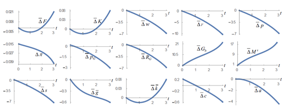
C. A rise in the household propensity to use gold
We now study the effects of the following rise in the propensity to use gold  The simulation results are plotted in Figure 4. As the household propensity to use gold is increased, the representative household tends to hold more gold in association with increasing gold price and gold-use costs. The government holds less gold and the economy has less physical wealth. It should be noted that, as in our approach the total gold is fixed, an enhanced preference for gold makes the household hold more gold. The money supply is reduced. Capital stock and output fall. The wage rate, price of the good, gold-use cost and gold price are all increased. The inflation rate is slightly increased. The consumption level rises. Total wealth rises.
D. A rise in the total factor productivity
We are now concerned with how total factor productivity affects economic growth. We now increase total factor productivity as follows: 
 The simulation results are plotted in Figure 5. As productivity is enhanced, the output level, national physical capital and wage rate are increased during the simulation period. The gold-use cost is increased, and the gold price is reduced. The inflation rate is reduced. The rate of interest is increased, and the price level is reduced. The household holds less gold and the government holds more gold. The money supply is expanded. The household consumes more and holds more total wealth.
E. The impact of the propensity to save
We now examine what will happen when the propensity to save is increased as follows:  . The simulation results are plotted in Figure 6. As the propensity to save is enhanced, the output level and physical capital are both increased. Both the wage rate and the rate of interest are reduced. It should be noted that, in the standard neoclassical growth model without gold, the change in directions of the wage rate and the rate of interest are the opposite when the propensity to save is changed. The gold-use cost and the gold price are decreased. The inflation rate is lowered. The household owns less gold and the government holds more gold. The money supply is expanded. The household consumes less and holds more total wealth
F. A rise the output elasticity of labor
We now examine what will happen when the output elasticity of labor is increased as follows: 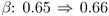 .The simulation results are plotted in Figure 7. The change in the parameter means that the share of labor cost in total cost is increased. It also means that the share of physical capital cost in total cost is reduced. The output level and physical capital are both reduced. Both the wage rate and the rate of interest are reduced initially and then increased. The total wealth is reduced initially and then increased. The gold-use cost is reduced initially and then enhanced. The gold price is increased. The inflation rate is enhanced. The household owns more gold and the government holds less gold. The money supply is reduced. The household consumes less. The household initially owns less total wealth and then more.
Concluding Remarks
This paper introduced money and gold into the Solow growth model. The study proposed a dynamic interdependence between gold distribution between monetary and non-monetary uses of gold, the gold price, money demand and supply, inflation, physical capital accumulation, wealth accumulation, and production. That way, the model determines money and price dynamics under the gold standard in the one-sector neoclassical growth model. The model was built upon a few approaches in the literature on the theory of economic growth. The production sector is based on the Solow model. The gold standard and price dynamics are based on Barro (1979). Household behavior is based on Zhang’s approach, which in turn is based on the traditional MIU model. The model integrated the ideas of these approaches within a compact framework. Through simulations, we show that the economic system has a unique unstable steady state. The study conducts comparative dynamic analysis regarding changes in some parameters.
As this model is built on many strict assumptions, we may generalize it and extend it by relaxing some of these. For instance, we may generalize the model by using more general functional forms for production and utility. It is also possible to extend the model by taking account of household heterogeneity. It is also important to generalize the model within a framework of heterogeneous sectors. This study does not take account of risks in different markets. Gold is often kept as a way of diversifying risks. A further understanding of dynamics in the gold market requires introduction of speculation and volatility. Although this study treats the gold supply as fixed, the supply of gold may also be derived from profit optimization in the gold mining industry in a framework where gold ore is exhaustible (e.g., Bordo & Ellson, 1985 and Dowd & Sampson, 1993).