English (pdf)
 Article in xml format
 Article references
 Send this article by e-mail
 Cited by SciELO
  Cited by Google
  Similars in
SciELO
Similars in
SciELO  Similars in Google
 Permalink
Introduction
In Labor Economics, the study of stress is a new field of research that allows incorporating methodologies and theories used mainly on studies in traditional topics such as quality and duration of employment. Thus, the theoretical model “leisure-consumption” widely used in Labor Economics that identifies the participation of people in the labor market becomes relevant for this investigation. It allows us to know how economic agents choose between a direct and indirect utility and depending on his dedication it bases the appearance of stress. The job stress directly affects the productivity of the worker (Halkos & Bousinakis, 2010), when it rises to levels not tolerable. According to the II Occupational Health and Safety Survey presented by the Ministry of Labor of Colombia (2013), psychosocial risks (stress) are generated in activities of attention to the public, postures that produce fatigue or pain, monotonous work and changes in the requirements of the task just to mention some of its causes.
Accordingly, it establishes the multidimensionality of the concept. Factors such as excessively demanding work, lack of time to complete tasks, lack of clarity about the role of the worker, imbalances between the demands of work and the worker’s competence are linked to this condition. However, there are also related factors such as lack of influence in the way in which the work is carried out alone, especially if it faces the public. The lack of support from management and colleagues, psychosocial harassment in the workplace, unfair distribution of work, rewards, promotions or career opportunities, ineffective communication and poorly managed organizational change, end up completing the details of the factors that explain the job stress. Between 2009 and 2012, the events derived from these risks presented an increase of 43%, mainly with anxiety and depression. In order to reduce the rate of illness or work accident caused by stress, the Colombian Security Council (CCS, in Spanish) joined the campaign of the European Agency for Safety and Health at Work “Healthy jobs: manage stress”. These efforts drive to thinking about the importance of approaching studies that penetrate on this condition.
The stress category is proposed by Lazarus and Folkman (1984) in his transitional model. These authors concluded that the stress results of a transition between a person and a condition to be treated in a defined environment. Here, this concept gains relevance since it affects the welfare of the population. Therefore, it is important to provide metrics that lead to its identification. In methodological terms, this research proposed a Job Stress Index (JSI) considering the existing heterogeneity between cities in terms of supply and demand of employment (unemployment) and incorporating the fuzzy sets measurement method. Data is collected from the Great Integrated Household Survey 2018 (GEIH, in Spanish), it is built by the National Administrative Department of Statistics (DANE, in Spanish). The government entity implements a probabilistic, stratified, multistage and conglomerate-related sample design, through which it assures representation for the national territory (Direction of Methodology and Statistical Production -DIMPE-, 2018, p. 7).
The data have a methodological clarity with which the employed and unemployment population can be identified in each of the 23 principal cities. Meanwhile, the population analyzed is defined as individuals that are employed and being between 16 (age considered as the time when they conclude high school) and 62 years old (retirement age for men). The result is a sub sample of 154817 observations representing 7683890 individuals. Once the JSI is constructed, we segment the index by quantiles in order to define three categories of this variable: high-stress, moderate-stress and low-stress. Besides, this research advances in the identification of the socioeconomic and labor characteristics that affect, on probabilistic terms, in its appearance. A multinomial probit type model is estimated. In effect, this research provides a measure of job stress in order to quantify it. The research hypothesis is defined as: job stress presents heterogeneity between regions (principal cities) and, there is no correlation that evidences that the labor dynamics within these (employment or unemployment) explain the job stress. The result leads to exploration about the individual characteristics that would explain the heterogeneity, being a microeconomic study.
This paper is organized into four sections. The first section is the review of literature that addresses the issue of job stress and its identification as a topic that has been studied mostly by the medical and social sciences compared to economy. Subsequently, a theoretical framework is presented, where the consumption-leisure model justifies the appearance of stress by the inequality in the first order condition in the model. A third section offered the empirical strategy, which shows the source of the dataset, the description of the variables used for the construction of JSI and the specification of a probabilistic econometric model to quantify the stress levels of the employed population. The next section presents the main results of the econometric exercise and the conclusions, limitations and recommendations are submitted at the end.
I. Literature Review
The factors associated with stress represent a certain complexity, since its causes are determined by psychological and physical factors that are not uniform to the participating population in the labor market. In this sense, this literature review documents academic findings around this condition, specifying that since it is not a study of causal relations, the exposure of the methods employed by these authors, their postulates and theoretical definition of stress contribute with elements that allow to understand characteristics, most of them observable, that will be introduced in the econometric analysis.
Freeman (1977) introduced the job satisfaction as a measured binary between the relation of satisfied or unsatisfied. It leads to behaviors that create negative labor dynamics such as resigning from the position and high rates of job mobility. Nevertheless, although the employed methodological component makes inferences about job satisfaction, its results contribute with evidence of two control variables which are of interest for this research, since they explain the appearance of job stress. The first variable is considered finding a new job, in which the author establishes a negative effect and the second variable as a responsibility of the employee, which was not statistically significant, explained to the extent that the greater the motivation of the employee the lower the probability of resigning.
On the other hand, Booth (1979) proposed a hypothesis that there are no marital problems due to the stress produced in the households as a result of the hiring of female employees. This research suggests that taking stratified samples of households in Canada and carrying out a distinction by gender, the author carried out a series of interviews and medical examinations to determine whether this population suffered from symptoms that would determine stress, such as colon diseases or frequent head or chest pains. Based on multiple regressions and an analysis of the existing correlations between job-related activities, marital relationships and stress-related diseases, it was established that there were no differences between couples in which the wife works and the one who stays at home.
Kolvereid (1982) analyzes the different factors that lead to job stress, focusing on organizational environment and occupational differences among sectors. The author finds that regarding the organizational environment, there is evidence that relationships with employers, the work environment and performance requirements are the main sources of job stress. Regarding occupational differences, the jobs in which people are exposed to a greater vigilance produce more stress in relation to people who have greater independence in their jobs. Another interesting aspect in this research is based on establishing that physical effort and high job competitiveness between co-workers are factors that explain the appearance of stress.
Heaney et al. (1993) contribute with interesting evidence from the field of organizational behavior. Analyzing the effect that interventions in occupational health produced on the stress of 1100 workers of the manufacturing sector, they found that industrial relationships between employees and employers led to joint solutions to relieve stress, since the fact of involving workers in the projects of occupational health improved the perception that employees had about employers, as well as the climate of participation within the company of the sample. This is one of the strongest conclusions of the study: substantial improvements in work relationships and labor climate had a positive influence on the levels of depression in the labor force.
A macroeconomic perspective, the research carried out by Fenwick and Tausig (1994) identifies the influence of certain variables in this field on stress.
The authors used the Survey on Quality of Work to labor force in the United States between 1973 and 1977 and a model of structural equations to conclude that the unemployment rate produces indirect effects on work conditions because it makes workers feel fearful of losing their job. In this sense, they also identify that recessions and variations in the economic cycle have an influence on individual stress due to, according to the context, people can be forced to change their work routines, which can increase the exposure to stressful situations such as longer working days per week.
Hernández et al. (1997) build a systematization of the different dimensions of job stress from the field of clinical sciences based on the Questionnaire on Work-related Stress (CUEL-34), with which they calculate the Index on Stress Reactivity. The authors apply the questionnaire to 106 workers of a Spanish publisher and by means of a factorial analysis they contrasted the relations between responses and physical conditions associated to stress such as level of cortisol and cholesterol, finding significant correlations between increases in the levels of cortisol, cholesterol and other substances related to stress to the extent that responses to the tests indicated a greater exposure to stress, due to factors such as work environment, workload, sense of belonging towards the job, job satisfaction, demands on oneself, among others.
Gamero-Burón (2010) estimates the costs of job stress on the Gross Domestic Product (GDP) of Spain from the variable lost workdays. Employing data of the Household Surveys and taking into account logistic regressions and regressions by Ordinary Least Squares (OLS) to estimate the differences between stressed wage earners and the ones who are not regarding work absences, controlling for the occupational levels of each job and taking into consideration the conditions of each region, the author specifies that around 0.11% of the GDP is lost due to low productivity created by job stress. In times of crisis, this suggests a significant amount, for which the author recommends that companies adopt strategies to decrease stress in workers.
Atalaya (2001) reviews different concepts of stress and job stress in literature. There is a consensus about stress being the biological consequence that the body assumes due to physical and emotional requirements demanded by the environment; in this way, the concept is also extrapolated to the work environment. People react differently to these requirements, but the key is to assume the pressure as a constant and create therapies that allow to relieve the load before it results in symptoms such as the increase in blood pressure, cardiovascular and digestive problems. Emotional requirements that jobs demand need a better organizational environment in the companies, since the author agrees with literature that organizational factors are the main causes of job stress. Consequences of stress at work are also reflected in the worker’s productivity, considering that that sense of achievement, self-perception and confidence decrease to the extent that stress increases. Because of this factor, companies must increasingly guarantee better work conditions for employees, so they feel comfortable and can better control the pressure demanded by the corporate world.
Oswald (2002) studies the determining factors of job stress after a comparative analysis between the United States and Europe from 1970 to 2000 and suggests that work satisfaction has an inverted-u shape as age advances, which is when women enjoy more their jobs than men. The author also identifies that the factor that produces more satisfaction is the one related to employment security. On the other hand, he mentions that in relative terms, income is a source of job satisfaction and that in industrialized countries people enjoy more their jobs; however, a decrease in the following decades has taken place causing job stress and a loss in the balance between work and family life.
Houtman et al. (2008) present a review of the main concepts approached by the definition, causes and impacts of job stress. In this review, the organization highlights that the perception of people about environmental, social and personal factors has an influence on stress generation and therefore, the measurement of this phenomenon must include these dimensions at individual and collective levels around the organizational environment. Meanwhile, one of the most interesting observations of this work resides on the biological consequences of stress and its influence on the performance of workers, since the main loss to organizations is productivity decrease. Additionally, the study by Durán (2010) analyzes the factors that cause job stress based on the review of the organizational environment. The author finds a relation between the increase of competences and physical, mental and emotional requirements that organizations demand of their employees with the appearance of stress symptoms and work addiction.
Jung and Yoon (2014) analyze the relations between emotional labor, emotional imbalances, job stress and intentions to rotate (understood as changing working hours or the assignment within the company) of the employees of family restaurants or companies associated with the sale of prepared food in Korea. They applied a study to 338 workers of these restaurants and by means of the development of a 50-question study that included questions about their feelings of interactions with consumers and employers, and corporate environment. The authors applied factorial analysis and the structural equations method to find that emotional labor was increasingly related to emotional imbalances, job stress and rotating attempts.
Even so, the job stress is the factor that most affects the decision to change positions inside the company.
Modekurti-Mahato et al. (2014) review the impact of emotional labor in job performance. In this way, the authors focus on job stress associated with the corporate environment for the service sector in India. In their work, they analyze 411 employees of the service sector and by means of the application of a questionnaire; they estimated an index that through a hierarchical scale determines the stress level of each employee. The indicator reflects that emotional labor is positively correlated to job stress and the organizational environment of the company. These correlations are significant and resulted from conventional regressions using the OLS. Meanwhile, an additional contribution of the authors is that there is a difference of stress associated with emotional labor in married women in relation to other types of workers in the sample.
Ruiz-Pérez et al. (2017) carry out an analysis around the socio-economic causes of stress. In this way, they carry out the exercise of reviewing the effect of recession in 2011 on mental health in Spain. The authors are based on the hypothesis that financial crises are associated with a greater exposition to collective stress. To confirm this hypothesis, the authors carry out a study for two periods based on the National Health Survey performed by the Spanish government, one before recession (2006) and the second one after recession. These included semi-balanced samples and psychic morbidity as the dependent variable, understood as mental illnesses related to stress. Socioeconomic, financial, psychosocial, labor market and State-related services were reviewed.
In this sense, by means of a multilevel logistic regression, it was found that the greater investment (or expenditure) in health per capita, the greater stress levels reflected in diseases. In the same way, precarious nature of the job and the poor conditions of the macroeconomic environment during the crisis caused stress to workers, for which the authors suggest that the government should preserve and increase health investments in times of crisis. This, with the purpose of supporting the most vulnerable people, so they can have access to the health system and obtain the psychosocial support they need to bear with the crisis and therefore, avoiding increases in the risk of having poor mental health.
In this literature review, the greatest job stress implications are present in the psychological and physical consequences that it produces over people (heart disease, depression and low self-esteem) and in the productivity loss of organizations (low performance, decrease in individual and group achievements); for which literature suggests that is the responsibility of organizations to implement occupational health programs that allow decreasing stress through improving work environmental conditions. This is achieved by means of the participation of employees in interventions, constant monitoring to teamwork and stimuli for employees with the purpose of reinforcing their sense of achievement and keeping their self-esteem high. However, no studies that focus on the determining factors of its appearance or clear measurement rules have been identified. So, this methodological approximation from the field of economic sciences becomes the main contribution of the research.
II. Theoretical Framework: The Classical Model Leisure-Consumption
The Job stress is the result of the disparity (inequality) between direct compensation produced by carrying out a remunerated economic activity and the dedicated time to leisure activities (indirect compensation); inasmuch as not producing a satisfaction level in accordance with the requirements and the time destined to carry out the work, for instance, together with organizational environment factors, the appearance of overwhelming situations that create psychosomatic reactions or psychological disorders is inevitable.
Currently, the most used stress model in psychology is the transactional model proposed by Lazarus and Folkman (1984). For these authors, stress is the result of a transaction between a person and a situation to deal with in a defined context. The individual, who has established objectives in relation to a situation, must anticipate the dynamic evolution of this situation with the purpose of establishing the balance between the resources at his disposal and the demands imposed by the situation. When the individual estimates that this balance is unfavorable for him in relation to his objectives, he develops stress. Is it worth mentioning that for these authors, a situation refers to a configuration of the environment?
Between the environmental or situational conditions faced by the individual, the demanded tasks to a worker in the frame of this contractual activity appear, as well as the authority, dependence in terms of resources, danger seen as the possibility of suffering from damages or losses, among others Lazarus and Folkman (1984). Therefore, it is supposed that stress will have physiological reactions, changes related to social behavior, somatization, disease, among other consequences (effects) on the individual. This allows to base the argument that stress is an individual cognitive process. In fact, job stress triggers when there is an imbalance between the perception of a person about the restrictions imposed by his environment and the perception or his own resources to deal with them. In this way, if this evaluation process is psychological, the effects of stress are not only of a physiological nature, considering that it affects physical health, wellbeing and the productivity of the person who suffers from it (Burón, 2010).
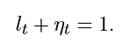
The etymological basis of stress presented previously allows to develop a proposal of conceptual articulation with the field of labor economics. The choice made by the agent about the time that he/she destined to carry out work-related and everyday activities is clearly supported by the analytic reviews of the basic labor model (leisure-consumption). Being these factors mutually exclusive, the imbalance of the first order conditions of the model, suggests the appearance of job stress. To submit the aforementioned to a test, this research takes parts of the mathematical development presented by Wickens (2011, pp. 33-35). The basic extension of the model begins with the choice that economic agents make about the time distribution in leisure activities (l t ), which provides an indirect utility to the individual and, labor (η t ), whose utility is direct in the sense that remuneration to his productivity (salary) is immediately reflected in the capacity to purchase consumption goods. Nevertheless, the natural time restriction is established as one of the most important conditions in the development of the model, which for the sake of practicality matters, literature suggests it should be normalized to one, being as follows:
 (1)
(1)
Immediate utility that leisure and labor report to agents complies with the classical conditions of a utility function, this means, as the agent destinies more time to carry out work-related activities (leisure), his instant utility increases, but not indefinitely, although not indefinitely, considering that when reaching a saturation point, utility is increasingly lower and therefore, it decreases:
 (2)
(2)
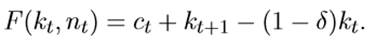
The model solutions require introducing a second restriction with which the agent is faced. Assuming that labor is one of the productive factors employed by the economy (company) and considering that the production function is neoclassical without introducing technology, in order not to involve the component of efficient labor and of technological shocks, this restriction is determined by the productive factors: capital (k t ) and labor (η t ) as follows:
 (3)
(3)
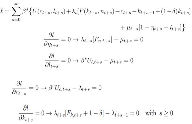
Equation (3) establishes the relation between the productivity of the company, consumption level of consumers and available capital accumulation in the following period, considering a rate of capital depreciation, which represents the natural wear or replacement. In this way, based on the three previous equations, the development of the model implies the inclusion of the dynamic optimization method by Lagrange (intertemporal), whose first order conditions are key to establish the theoretical basis on which this research relies:
 (4)
(4)
The solution to the model appears when combining the first order condition of labor (η t+s ), leisure (l t+s ) and consumption (C t+s ), given that carrying out the algebraic estimations, the equality between marginal utility of leisure and marginal utility of consumption weighted by the marginal productivity of labor, commonly known as salary, is obtained:
 (5)
(5)
From the result of Equation (5) it is possible to detect the appearance of job stress. When supporting that as the agent employs a greater number of hours to work-related activities (work) than to the rest of the everyday activities (leisure), his remuneration increases, but not indefinitely and will always be a lower rate until the point that it will reach a maximum peak (saturation). This result leads to the decrease of the marginal utility of consumption, therefore, the trade-off between labor and leisure is not compensated by the salary increase. Therefore, in view of the decrease of available time to carry out other pleasure-related activities, the agent experiences a loss of wellbeing to the extent that spending more time to work does not represent a remuneration in accordance with his effort and this also makes him more prone to interact in contractual environments that will inevitably affect his physical and mental health. Then, the rational choice of the individual should be to destine a little more time to recreational activities (leisure). This is mathematically expressed as follows:
 (6)
(6)
Regarding the compliance of the aforementioned theoretical assumption, the conclusion of the model is given when resolving the equation of Euler, which is the result of the fourth first order condition of the optimization process that contributes by explaining why job stress negatively affects the productivity of the economy (company). Nevertheless, the scope of the research is aimed in the estimating a job stress index and analyzing the conditions that might affect its appearance, instead of its effects on productivity, leaving the open possibility of developing future research around it.
III. Empirical Strategy
A. Database and variables
Data are collected from the Great Integrated Household Survey 2018 built by the DANE. The government entity implements a probabilistic, stratified, multistage and conglomerate-related sample design, through which it assures representation for the national territory (DIMPE, 2018, p. 7). The justification of its use is based on the methodological clarity with which the employed population can be identified in each of the 23 principal cities and on the detailed data section about employment of economic agents. Meanwhile, the population analyzed is defined as individuals that are employed and being between 16 (age considered as the time when they conclude high school) and 62 years old (retirement age for men). The result is a sub sample of 154817 observations representing 7683890 individuals.
The dependent variable corresponds to the JSI, whose construction forms part of one of the established objectives in this research. The fuzzy sets method was employed based on the consideration of seven binary variables associated to the quality and perception of employment; these variables would lead to job stress quantifying. These are: i) satisfaction with the current job, ii) received bonuses and compensations, iii) current working hours, iv) job stability, v) compatibility between the job and family responsibilities, vi) whether he/she is affiliated to social security and vii) he/she foresees funds he would use in the event of being unemployed (see Table 1A in the annex). Additionally, it is evident that there are cities that concentrate a greater or lower proportion of employed population, which made it necessary to explore a presumed relationship between labor dynamics and the index.
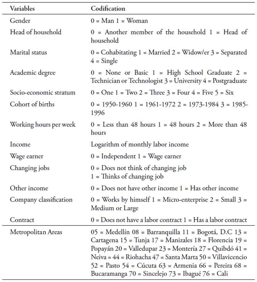
The explanatory variables were specified in 2 components. The first one was called job characteristics and variables such as weekly working hours, income resulting from economic activity (logarithms), whether the individual is a wage earner or independent, if he desires to change company, if the company is small, medium or large, if he has a contract of employment and if he has other income sources were evaluated. The second component allows to characterize the individuals and variables such as gender, whether he is the head of the household, marital status, cohort of birth, academic degrees and socio-economic stratum. The definition and codification of the explanatory variables are reported in Table 2A (annex) and the main statistical parameters can be seen in Table 3A (annex).
B. Fuzzy set measurement method
The fuzzy set method is employed to build an individual job stress index as an empirical strategy adapted to works oriented to analyze labor market statistics or the quality of life documented by Lelli (2001) ; Lemmi and Betti (2006) ; Bérenger and Verdier (2007). This approach follows the proposal by Desai and Shah (1988), who suggest that the social environment is an important factor in the measurement of privation. In this sense, the method allows to determine the level of belonging of individuals to a set (in this case, presenting job stress-related factors) by means of functions relating to a sense of belonging. The advantage of the method is the easy interpretation of the final weightings, considering the simplicity of the procedure, especially if it is compared to the methods that employ principal components or factorial analysis that require continuous quantitative variables in certain cases and the estimation of own values and correlations.
The mathematical formulation presented in this work follows Lelli (2001).
X represents the universe composed by individuals named as x i with i =
1,...,n, which have a vector of j attributes or characteristics such that j = 1,...,T. Now, A is a fuzzy subset of X, such that if x i ∈ A, the individual i does not suffer from the privation of any attribute. If the level of belonging of x i to A is expressed by a µ A function that can take values in the interval [0,1], then A would be a fuzzy subset. In this way, A could be expressed as A = {(x i ,µ A (x i ),x i ϵX)}. On its part, the µ A function that defines the level of belonging will be defined as:
µ A (x ij ) = 1, in case of not belonging to the subset A.
µ A (x ij ) ∈ (0,1), in case of partially belonging to the subset A. This is total or partial privation of some attributes, but not totally deprived of them. µ A (x ij ) = 0, in case of total belonging or membership to the subset A.
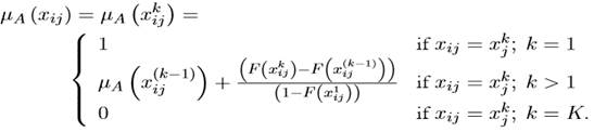
Where µ A (x ij ) is an individual measure of specific privation for the j indicator. In addition to this, Lelli (2001) recommends to use the cumulative distribution function, considering that it allows to avoid arbitrary definitions of thresholds to determine a sense of belonging. Likewise, unlike the other functional forms, the cumulative distribution does not require preestablishing limits to the sets and it is possible to obtain total scores and scores by dimension. In this case, according to the proposal by Cheli and Lemmi (1995), the function would be the following:
 (7)
(7)
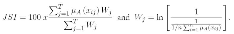
where k = 1,...,K is each one of the categories of the variable j (seven in this research) that explain the risk of privation, being K the lowest risk (this means,the best situation in relation to the variable j). F (x j ) is the cumulative distribution of the variable j, classified according to k. Once the functions that measure the level of belonging are obtained, the JSI is calculated as the weighted average of these in the following way:
 (8)
(8)
In this case, T represents the total of dimensions and W
j
the respective weighting, which is calculated as shown in Equation (8). Lastly,
 represents the fuzzy proportion of individuals with certain level of not presenting labor stress in relation to variable j. A simulation of a hypothetical situation is presented below. Table 1 presents the data of an example for 15 individuals, which uses, for simplification purposes, only five dimensions or variables. The following variables are included in the columns of the table with the respective numeral:
Satisfaction current job 0 = Satisfied 1 = Not satisfied
Satisfaction bonuses and benefits 0 = Satisfied 1 = Not satisfied
Satisfaction current working hours 0 = Satisfied 1 = Not satisfied
Job Security 0 = Does consider it 1 = Does not consider it
Compatibility between work and family responsabilities 0 = Compatible 1 = Not compatible
In this way, the economic agents with lower JSI would be the ones satisfied with their current job, receiving bonuses and compensations, are satisfied with the current working hours, consider they have job stability, that there is compatibility between work and family responsibilities, they are affiliated to social security and foresee the funds they would use in the event of being unemployed, with which the JSI would have a score of 100. On the contrary, the individuals under privation in each of the studied variables obtain a JSI score of 0. Indeed, taking the previous into account, it is highly important to highlight that this type of weighting refers to its awareness of the frequency, in such a way that it does not give great importance to the infrequent or rare stress-related characteristics. In this way, the result will be an individual job stress index, which when aggregated by different categories (in this case, metropolitan areas) will allow to enrich the analysis.
Table 1 Simulation Job Stress Index
| ID | City | (1) | (2) | (3) | (4) | (5) | µ(1) | µ(2) | µ(3) | µ(4) | µ(5) | W(1) | W(2) | W(3) | W(4) | W(5) | JSI |
|---|---|---|---|---|---|---|---|---|---|---|---|---|---|---|---|---|---|
| 1 | Medellín | 0 | 0 | 0 | 1 | 0 | 1 | 1 | 1 | 0 | 1 | 1.10 | 0.51 | 0.51 | 0.92 | 0.14 | 71.18 |
| 2 | Medellín | 1 | 0 | 0 | 0 | 0 | 0 | 1 | 1 | 1 | 1 | 1.10 | 0.51 | 0.51 | 0.92 | 0.14 | 65.45 |
| 3 | Medellín | 0 | 1 | 0 | 1 | 0 | 1 | 0 | 1 | 0 | 1 | 1.10 | 0.51 | 0.51 | 0.92 | 0.14 | 55.12 |
| 4 | Medellín | 1 | 0 | 1 | 1 | 0 | 0 | 1 | 0 | 0 | 1 | 1.10 | 0.51 | 0.51 | 0.92 | 0.14 | 20.57 |
| 5 | Medellín | 0 | 0 | 0 | 0 | 0 | 1 | 1 | 1 | 1 | 1 | 1.10 | 0.51 | 0.51 | 0.92 | 0.14 | 100.00 |
| 6 | Medellín | 1 | 0 | 0 | 1 | 0 | 0 | 1 | 1 | 0 | 1 | 1.10 | 0.51 | 0.51 | 0.92 | 0.14 | 36.63 |
| 7 | Medellín | 1 | 0 | 1 | 0 | 0 | 0 | 1 | 0 | 1 | 1 | 1.10 | 0.51 | 0.51 | 0.92 | 0.14 | 49.38 |
| 8 | Medellín | 1 | 1 | 0 | 1 | 0 | 0 | 0 | 1 | 0 | 1 | 1.10 | 0.51 | 0.51 | 0.92 | 0.14 | 20.57 |
| 9 | Medellín | 0 | 1 | 1 | 1 | 0 | 1 | 0 | 0 | 0 | 1 | 1.10 | 0.51 | 0.51 | 0.92 | 0.14 | 39.05 |
| 10 | Medellín | 1 | 0 | 0 | 0 | 0 | 0 | 1 | 1 | 1 | 1 | 1.10 | 0.51 | 0.51 | 0.92 | 0.14 | 65.45 |
| 11 | Medellín | 1 | 1 | 0 | 1 | 0 | 0 | 0 | 1 | 0 | 1 | 1.10 | 0.51 | 0.51 | 0.92 | 0.14 | 20.57 |
| 12 | Medellín | 1 | 0 | 0 | 1 | 0 | 0 | 1 | 1 | 0 | 1 | 1.10 | 0.51 | 0.51 | 0.92 | 0.14 | 36.63 |
| 13 | Medellín | 1 | 0 | 1 | 0 | 1 | 0 | 1 | 0 | 1 | 0 | 1.10 | 0.51 | 0.51 | 0.92 | 0.14 | 44.88 |
| 14 | Medellín | 1 | 1 | 1 | 1 | 1 | 0 | 0 | 0 | 0 | 0 | 1.10 | 0.51 | 0.51 | 0.92 | 0.14 | 0.00 |
| 15 | Medellín | 0 | 1 | 1 | 0 | 0 | 1 | 0 | 0 | 1 | 1 | 1.10 | 0.51 | 0.51 | 0.92 | 0.14 | 67.87 |

|
5 | 9 | 9 | 6 | 13 | ||||||||||||

|
3.18 | ||||||||||||||||
| Average JSI | 46.22 | ||||||||||||||||
Source: author’s calculations.
C. Multinomial probit models and econometric specification
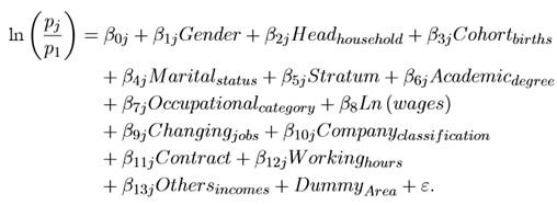
Multinomial discrete choice models are based on the utility theory of the economic agent. In this sense, considering as determining factors the socioeconomic and job profile characteristics that do not present endogenous problems, it is possible to quantify the probability of being stressed. Indeed, we segment the index by quantiles in order to define three categories of this variable: high-stress, moderate-stress and low-stress (see Table 4A in the annex). The dependent variable has a polynomial structure of the form Y = {1,2,3}, with probabilities of occurrence equal to p 1 = p(Y = 1), p 2 = p(Y = 2) and p 3 = p(Y = 3) = 1 − p 1 − p 2 and considering as a reference category the lower stress, the equation to estimate is the following:
 (9)
(9)
The discrete choice model estimated supposes a probit distribution. So, the basis of this empirical strategy doesn’t depend on the compliance of the assumption of Independence of Irrelevant Alternatives (IIA), as much as it must be proven that in case of eliminating one of the categories of the dependent variable, the estimated coefficients are not modified. For instance, if the categories of greater stress and moderate (excluding low-stress) job stress were considered, significant variations in the reported estimations considering both alternatives should not be obtained. The null hypothesis Small and Hsiao (1985) is: there are no differences between the estimated coefficients and the categories of the dependent variable, and it was rejected (Table 5A in the annex). Therefore, it can be concluded that the data adopt a normal distribution and a probit ordered multinomial model is estimated and the variables have not multicollinearity problems (Table 6A in annex).
D. Job Stress Index and Economic Inference
We estimated the JSI for the principal cities of Colombia, which concentrate a high proportion of the employed population in the country. In the 2018, the cities registered an employment rate of 58.6%; slightly lower than the one registered in 2017 (59.5%) and a little higher in relation to the national registers, 57.8% (DANE, 2018, pp 6-9). Table 2 reports the main statistical aspects of the JSI ranked from lowest to highest, reaffirming that the fuzzy sets method proposal validates the privation of the characteristics associated with job stress, and therefore, the lower score meaning more stress level. Meanwhile, employment and unemployment rates in 2018 are also reported in the last columns, in order to observe whether there are patterns between employment (unemployment) and job stress.
Table 2 Job Stress Index - Labor Market Measures 23 principal cities
| Cities | JSI | Labor Market | |||
| Observation | Mean | Deviation | Employment (%) | Unemployment (%) | |
| Medellín | 12157 | 80.35 | 23.14 | 57.70 | 11.70 |
| Barranquilla | 10032 | 71.28 | 26.67 | 59.60 | 8.50 |
| Bogotá | 10506 | 74.43 | 23.33 | 61.90 | 10.50 |
| Cartagena | 4718 | 76.97 | 26.83 | 51.70 | 8.70 |
| Tunja | 5968 | 73.52 | 25.53 | 54.50 | 11.30 |
| Manizales | 7772 | 75.20 | 23.59 | 52.80 | 11.20 |
| Florencia | 4907 | 78.48 | 23.62 | 51.80 | 13.00 |
| Popayán | 5369 | 65.20 | 26.59 | 52.70 | 10.90 |
| Valledupar | 5419 | 71.95 | 29.23 | 52.10 | 14.80 |
| Montería | 7363 | 68.28 | 32.43 | 57.40 | 10.00 |
| Quibdó | 1839 | 75.95 | 26.77 | 48.10 | 17.80 |
| Neiva | 6869 | 71.98 | 27.02 | 55.70 | 11.60 |
| Riohacha | 6459 | 66.71 | 27.35 | 53.50 | 14.10 |
| Santa Marta | 5095 | 72.01 | 28.60 | 54.50 | 8.40 |
| Villavicencio | 6291 | 81.12 | 22.77 | 58.10 | 11.90 |
| Pasto | 6337 | 61.28 | 29.18 | 58.90 | 9.00 |
| Cúcuta | 4338 | 69.78 | 28.36 | 51.00 | 16.30 |
| Armenia | 6357 | 66.20 | 27.28 | 54.80 | 15.60 |
| Pereira | 7019 | 82.46 | 22.55 | 59.30 | 9.10 |
| Bucaramanga | 7548 | 85.10 | 20.88 | 61.20 | 8.80 |
| Sincelejo | 7844 | 68.02 | 33.03 | 61.70 | 9.60 |
| Ibagué | 6433 | 77.17 | 26.65 | 56.00 | 14.20 |
| Cali | 8177 | 76.39 | 24.19 | 59.70 | 11.50 |
| Total | 154817 | 75.61 | 24.86 | 58.70 | 10.90 |
Source: author’s author’s calculations based on the GIHS 2018.
There are 14 cities with a JSI under the estimated mean for the 23 principal cities. Pasto reports the lowest index (61.28), which suggests that the employed population presents conditions that enables its appearance; followed by intermediate cities such as Popayan (65.20), Armenia (66.20), Riohacha (66.71), Sincelejo (68.02), Monteria (68.28), Cucuta (69.78) among others. On the other hand, Bucaramanga (85.08), Pereira (82.6), Villavicencio (81.12) and Medellin (80.35) reported a JSI of more than 80 points. Therefore, these four cities are the one with the least job stress and it’s possible that the labor conditions are positive for the employed population, but this assumption exceeds the scope of this research. Meanwhile, one of the context-related variables that can affect the appearance of job stress is the employment rate.
In a city where the unemployment rate is high, for instance, it is likely that employed people feel pressure to keep their current jobs regardless of the requirements of hours and the received remuneration for carrying out the activity, since changing jobs would not be easy. However, when analyzing the results of the JSI and the employment rate for the set of cities, there is not a clear relation that suggests that more employment less stress (see Figure 1).
Job stress, as identified in this research, according to the empirical strategy employed for its calculation and econometric inference suggests the existence of job stress in the labor market at the 23 principal cities of Colombia. In principle, the statement is supported to extend that the probability of presenting high-stress, moderate-stress and low-stress that depends on a set of pre-established characteristics (explanatory variables) is 17.19%, 27.85% and 54.96%, respectively. In view of this result, the statistical review of the variables in the three defined components (see Table 3) are the marginal effects of a multinomial probit regression model. Therefore, its correct interpretation results by multiplying the coefficient by 100.
Table 3 Marginal effects in the multinomial probit model for the JSI
| Job Stress Index | High-Stress | Moderate-Stress | Low-Stress | |
|---|---|---|---|---|
| Socio-demographic characteristics of the individual | Gender [1=Woman] | -0.0182*** | -0.0192*** | 0.0373*** |
| (0.002) | (0.003) | (0.003) | ||
| Head of household | 0.0127*** | 0.0169*** | -0.0296*** | |
| (0.002) | (0.003) | (0.003) | ||
| Cohort of births "1961-1972" | 0.0116*** | 0.0063 | -0.0178*** | |
| (0.004) | (0.004) | (0.005) | ||
| Cohort of births "1973-1984" | 0.0164*** | 0.0035 | -0.0200*** | |
| (0.004) | (0.004) | (0.005) | ||
| Cohort of births "1985-1996" | 0.0140*** | -0.0019 | -0.0120** | |
| (0.004) | (0.005) | (0.006) | ||
| Married | -0.0245*** | -0.0054 | 0.0299*** | |
| (0.003) | (0.004) | (0.004) | ||
| Separated-Divorced | 0.0316*** | 0.0276*** | -0.0592*** | |
| (0.004) | (0.004) | (0.005) | ||
| Widow/Widower | 0.0272** | 0.0030 | -0.0301** | |
| (0.012) | (0.013) | (0.014) | ||
| Single | 0.0071** | 0.0120*** | -0.0191*** | |
| (0.003) | (0.003) | (0.004) | ||
| High School | -0.0185*** | -0.0078 | 0.0263*** | |
| (0.007) | (0.008) | (0.009) | ||
| Technician/Technologist | -0.0340*** | -0.0175** | 0.0515*** | |
| (0.006) | (0.008) | (0.010) | ||
| University | -0.0349*** | -0.0239*** | 0.0588*** | |
| (0.007) | (0.009) | (0.010) | ||
| Postgraduate studies | -0.0320*** | -0.0414*** | 0.0734*** | |
| (0.008) | (0.009) | (0.011) | ||
| Social stratum two | -0.0185*** | -0.0054 | 0.0239*** | |
| (0.003) | (0.003) | (0.004) | ||
| Social stratum three | -0.0346*** | -0.0113*** | 0.0459*** | |
| (0.003) | (0.004) | (0.004) | ||
| Social stratum four | -0.0477*** | -0.0285*** | 0.0763*** | |
| (0.005) | (0.006) | (0.007) | ||
| Social stratum five | -0.0637*** | -0.0495*** | 0.1132*** | |
| (0.007) | (0.009) | (0.010) | ||
| Social stratum six | -0.0813*** | -0.0610*** | 0.1423*** | |
| (0.009) | (0.011) | (0.013) | ||
| Labor characteristics | Wage earner | -0.1905*** | -0.0385*** | 0.2290*** |
| (0.005) | (0.005) | (0.006) | ||
| Labor income (ln) | -0.0112*** | -0.0022*** | 0.0134*** | |
| (0.001) | (0.001) | (0.001) | ||
| Changing job | 0.4576*** | 0.0048* | -0.4624*** | |
| (0.003) | (0.003) | (0.003) | ||
| Micro-enterprise | -0.0035 | 0.0020 | 0.0015 | |
| (0.004) | (0.005) | (0.006) | ||
| Small | -0.0567*** | -0.0083 | 0.0650*** | |
| (0.004) | (0.006) | (0.007) | ||
| Medium-Large | -0.0988*** | -0.0115** | 0.1103*** | |
| (0.004) | (0.006) | (0.006) | ||
| Has a contract of employment | 0.0941*** | 0.0350*** | -0.1290*** | |
| (0.005) | (0.007) | (0.007) | ||
| Works 48 hours | -0.0342*** | 0.0126*** | 0.0216*** | |
| (0.003) | (0.003) | (0.003) | ||
| Works more than 48 hours | 0.0230*** | 0.0112*** | -0.0342*** | |
| (0.003) | (0.003) | (0.004) | ||
| Has other income | -0.0105*** | -0.0079** | 0.0185*** | |
| (0.003) | (0.003) | (0.004) | ||
| Dummy Metropolitan Area | YES | YES | YES | |
| Probability | 17.19% | 27.85% | 54.96% | |
Note: significant coefficient at * for p<0.1, ** for p<0.05, *** for p<0.01.
Source: author’s calculations based on the GEIH 2018.
The socio-demographic characteristic component begins with the presentation of two outstanding results. Women have a lower probability of experiencing high job stress. Results show that it is 1.8 percentage points (pp) less in comparison to men. While being a head of household increases the probability in 1.27 pp of experiencing a high JSI. The previous statement contributes with evidence that in the labor market, gender and role differences persist in participative indicators such as salaries (gaps), position in the household and now, stress levels.
When examining how age and marital status affect job stress levels, results were statistically significant, but not very important. Results support that people born between 1973 and 1984 present a higher probability of experiencing low job stress, while young people (born between 1985 and 1996) experience a lower probability. In other words, the young people are more stressed. Now, being single, separated-divorced or widower increases the probability in 0.7 pp, 3.2 pp and 2.72 pp respectively, of experiencing high job stress, while being married decreases the probability.
Results of social stratum show that the greater the individual’s social stratum the lower the probability of experiencing high job stress levels, since it reduces as this variable of social position increases, in which its range fluctuates between 1.85 and 8.13 pp. This result can be supported to the extent that the stratum reflects the social position and/or acquisitive power of individuals and therefore, would not experience stress symptoms caused by the uncertainty about their income source in case of being unemployed or desiring to change jobs. Besides, the educational level explains the job stress. More education is associated with a low probability of being with high job stress, the results in the first column of Table 2 indicate that the probability decreases between 1.85 to 3.49 pp compared to the people who have no education level.
Work-related characteristics not only contribute with evidence that support the appearance of job stress considering the articulation of the basic labor model Leisure-Consumption, but they also allow us to observe the more relevant coefficients and the ones with a statistical significance of 1%. The wage earners have established a contractual relation, whose common denominator is the fixating of the contract period (permanent or indeterminate) and remuneration for the hired service. This statement implies a greater job security and a constant income flow which together are associated with a decrease of 19.05 pp in the probability of experiencing high job stress levels in relation to those who are not wage earners, this means, those who work on their own or are independent. However, the labor formality does not necessarily imply having a contract of employment, whether it is verbal or written, and in this sense, it is evident that those who have a contract of employment increase in 9.41 pp the probability of experiencing higher stress levels, explained by the fact that greater formality implies a greater number of responsibilities.
Results for the variable income (in logarithms) show that its increase produces a decrease of 1.34 pp in the probability of experiencing higher levels of job stress. An implication resulting from the salary increase as a response to a better compensation for the time destined to the work, is reflected in a fall of consumption utility. Then, to destine more time in work-related activities, even at the expense of a salary increase, results causing a loss of wellbeing. On the other hand, the feeling of wellbeing within the work environment, without specifying its cause, and that leads to consider the possibility of change jobs, is associated to an increase of 45.76 pp in the probability of experiencing higher stress levels, being this, the most important coefficient in the study. This analysis allows to indicate the importance of including alternatives that seek to decrease the condition within jobs, which opens a field of action for the elaboration of academic studies that will allow to know the decision of an economic agent to continue in a job.
Working hours represent an essential interest in labor market research, since increasing working hours, even when a salary increase takes place, has a negative influence in the individual’s wellbeing. This is supported when finding that working more than the established hours by the Colombian Law (48 hours) increases the probability of experiencing higher stress levels in 2.30 pp, in comparison to those who work less than 48 hours; while, working exactly 48 hours a week decreases that probability in 3.42 pp. This suggests that the ideal time to perform work-related activities would be around 48 hours a week, if the strategy is aimed at lowering down the stress of the employed population.
Finally, the size of the company explains the job stress. In larger companies there are better positions, which in certain way, would allow to balance the assigned schedules and responsibilities. In this sense, the proposed model suggests that in small, medium or large companies, the probability that the employed population experiences higher levels of job stress decreases in 5.67 and 9.88 pp; which supports the previously outlined assumption.
Conclusions, Limitations and Recommendations
Job stress is identified with more clearly if aspects related to the individual’s health are analyzed, as it has been identified in literature. Nevertheless, recognizing work conditions as demographic that are related to this phenomenon, becomes a research field that from the perspective of economic sciences has not been reinforced, possibly because of the limitation of information sources. Indeed, the information reported in population surveys do not usually develop extensive modules on labor force and in turn on issues of health of individuals.
Job stress levels can lead to increases in the productivity of the individual, since recognizing that labor markets increasingly assign a greater number of responsibilities that create positive organizational synergies regarding results. However, the main objective of this research was focused on analyzing the conditions that affected the probability of increasing or reducing job stress levels, because it certainly prompts behaviors that risk human health and social relationship of the employed person. So, this research partially adapts a broadly used methodology to calculate indicators of employment quality. Thus, it becomes the first methodological attempt that deserves to be further reviewed considering the possibility of introducing variables in the health of the individual, since they have an influence in its appearance. However, given the employed source of data, it was not possible to comply with such requirement, setting in this way an academic challenge for future research.
The flexibility based on new assumptions in the basic theoretical model of labor market leisure-consumption, allows to articulate the etymology of the term job stress and its possible appearance in the labor market. The analytical development of the model allowed us to establish that the greater time destined to execute work-related activities, the lower the utility resulting from consumption to the extent that the salary would not compensate this additional time to everyday activities (Leisure). Then, when finding statistical significance for the variables of the labor component such as working hours, having a contract of employment, classification of the company, among other variables, it possible to suggest the importance of encouraging work regulating frameworks that provides incentives, not only according to the salary but also oriented to maintaining a number of pre-established hours and additional time to execute complimentary activities.
The hypothesis of this research is empirically contrasted when analyzing the labor dynamics and the stress index found. In this way, it is observed that although stress is a heterogeneous phenomenon between cities, there is no statistical evidence to support a correlation between stress and employment rate, for example. This is important in that it is expected that the greater the available labor force, the pressure to keep their jobs may lead economic agents to perform extra activities not necessarily influence their economic welfare in favor of keeping their jobs. However, this precision should be explored more thoroughly in future research.