English (pdf)
 Article in xml format
 Article references
 Send this article by e-mail
 Cited by SciELO
  Cited by Google
  Similars in
SciELO
Similars in
SciELO  Similars in Google
 Permalink
Introduction
The National Institute of Statistics and Censuses of the Argentine Republic (INDEC, in Spanish) publishes price and quantity indexes of foreign trade at aggregate level and disaggregated by the main classification of goods for exports and economic uses for imports. These data are insufficient to make more disaggregated sectoral analyzes, to relate them with other variables such as output or employment, and to make international comparisons.
Thus, the aim of this paper is to present a methodology to estimate the international price indexes of Argentina by economic sector based on the International Standard Industrial Classification (ISIC) Revision 3.1 (United Nations, 2005). Then, this methodology is applied to the quarterly data of Argentine imports and exports from 1996 to 2016, both at the aggregate level and at 2-digit of the ISIC classification. The accuracy of the methodology is verified by comparing the results with the official estimates (in the case of the aggregate level) and with the data from Brazil (in the 2-digit sector). Finally, sectoral price indexes are used to obtain export and import volumes in order to analyze the recent evolution of the country’s foreign trade.
Given the lack of a survey to collect prices, we use unit values to build price indexes using data based on the 8-digit disaggregation of the Unified Mercosur Nomenclature (NCM, in Spanish). We reviewed several authors to determine the methodology for the treatment of the sample, which is crucial to deal with composition effects. We estimated Laspeyres, Paasche and Fisher indexes because official data in Argentina and Brazil are based on those formulas.
The paper is organized as follows. After this introduction, we analyze the importance and possible uses of the sectoral price and quantity indexes in external trade and the current limitations due to their absence. Next, we describe the methodology for the treatment of the sample. In the third section, the indexes are calculated and compared with the official estimates of the INDEC and the Institute of Applied Economic Research (IPEA, in Portuguese) of Brazil, and contribution of each economic activity to foreign trade growth is analyzed using the quantity indexes. Finally, we comment the concluding remarks and other possible uses for future research.
I. The current foreign trade data of Argentina
The price indexes of foreign trade are an indispensable tool for several reasons. They are used to deflate the value series of the trade flows to obtain the volumes traded (IMF, 2009). Likewise, these indexes are vitally important to study the influence of international trade on domestic inflation and the vulnerability in the presence of external shocks (U.S. BLS, 1997). At the sectoral level, they allow for a more complete overview of the productive specialization and the trade gains given by the degree of openness of the economy (Gaulier et al., 2008). In addition, these indexes are necessary to study inter and intra-industry trade, the long-run trends in prices and terms of trade and to estimate the foreign trade elasticities (U.S. BLS, 1997).
Currently, INDEC publishes values, prices and quantities indexes for imports and exports (and terms of trade) at the aggregate and low disaggregation levels. Exports are decomposed by main classification of goods (Primary Products, Manufactures of Agricultural Origin, Manufactures of Industrial Origin and Fuels and Energies), while imports are differentiated by economic use (Capital Goods, Intermediate Goods, Fuels and lubricants, Spare parts of capital goods, Consumer goods and Passenger motor vehicles).1 Since the disaggregation differs between exports and imports, it is not possible to get the sectoral trade balance.
In order to elaborate the price indexes with deeper disaggregation, we used the monthly database provided by INDEC, which collects export and import values (in dollars) and weight (in kilograms). The database also specifies the origin and destination of trade flows and the 8-digit tariff position corresponding to the NCM classification, through which it can be identified its correspondence with the ISIC classification. An index based on this later classification allows sectoral studies of foreign trade with the same disaggregation for imports and exports. Likewise, the ISIC is an international classification system, so it also allows comparison between countries. In the case of Argentina, other variables, such as employment or output, have this same classification making possible to perform wider analyses about different industries.
Regarding the possible use of the kilograms of the products to build a volume index, the issue is that the price depends more on the quality of the product than on its weight, which can generate serious composition effects. Indeed, the United Nations (1981) show that changes in the weightings of each product can lead to significant biases (sub or over-estimation) in prices’ change of rate due to a composition effect. The International Monetary Fund (IMF, 2009) recommends that when there is a difference between the economic estimates and the customs data, the economic estimation of the volumes must prevail. Even, the U.S. Bureau of Labor Statistics (1997) points out that it is not possible to keep a strict control over the physical trade quantities, so the volumes must be estimated deflating values by price indexes.
Therefore, unit values (ratio between the value and kilograms) are used to create a price proxy since there are no surveys or price records of the trade flows in Argentina. However, using unit values to construct price indexes has its own drawbacks. Although the United Nations (1981) affirm that, the deviation due to the use of the unit values is bearable, Silver (2007) concludes the opposite after analyzing the data of Germany and Japan. In addition, when using unit values as a proxy for prices, some limitations emerge with regard to the distinct features of the product (e.g. differences in quality). For this reason, calculating unit values is not a big problem in non- differentiated products, but it is really an issue in differentiated ones (INDEC, 1996).
For all this, it is essential to perform an exhaustive treatment on the database. First, following Hallak’s suggestion (Hallak, 2006), products of the same tariff position are classified by origin and destination to identify quality differences. In fact, the United Nations (1981) consider that breaking down by region allows us to capture the differences in product varieties in the same tariff position. Secondly, an exhaustive corrective treatment of outliers is performed, which is described in the next section.
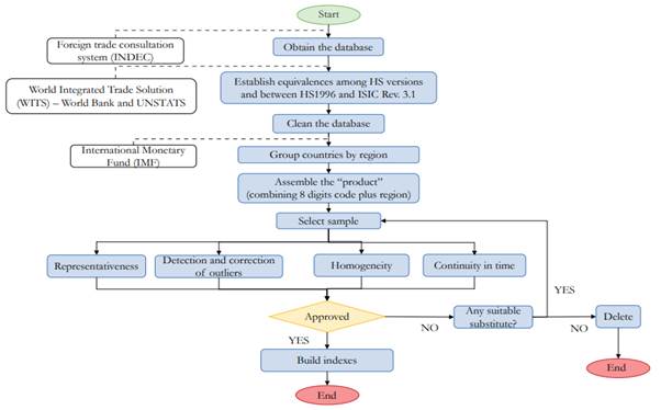
II. Methodology2
The primary data source is provided by the Foreign Trade Consultation System of the INDEC. These data are disaggregated by tariff position up to eight digits of the NCM by means of which we can identify the correspondence with the ISIC. The first six digits of the NCM classification is based on the Harmonized System (HS), but the classification system changed three times during the period covered by our study (2002, 2007 and 2012), so it is necessary to bring all the items to the same HS version. The most recent versions of the classification usually tend to have a deeper disaggregation of the items (Bernini et al., 2018); hence, all the items were taken to the HS 1996 version to impute the correspondence with the ISIC rev. 3.1.
Once we obtain all the series in the same classification, the first step was to eliminate all those observations prior to 1996 due to the presence of missing values in the data. In addition, trade flows with values or kilograms equal to zero were dropped. Finally, the observations in which the country of origin or destination is a region of Argentina, duty-free or indeterminate zones were eliminated as well. Tariff positions of services were not considered because lack of information about weight data (Kg).
After cleaning the database, the countries were grouped in seven regions according to the IMF classification3. We did so to homogenize countries with similar economic characteristics in order to simplify the treatment of outliers and to solve the discontinuity in data of the individual trade flows of each country. It is also a way to discriminate qualities, claiming that those destined to or coming from advanced economies tend to have a higher quality (Hallak, 2006; Byrne et al., 2017).
As the objective of this paper is to calculate the aggregate and 2-digit ISIC price indexes of exports and imports, we defined a unit of analysis based on the lowest possible level of disaggregation to reduce the composition effect and to have the possibility of calculating price indexes by 4-digits sectors. Thus, taking advantage of the correspondence between the ISIC and the NMC, the sector code was created unifying the four digits of the ISIC and the first four digits of the NCM to individualize the 8-digit products that compose the 4-digits ISIC sector. A second grouping was to divide the products by region. In this way, two products with the same 8-digit code are considered as different products if they come from or are destined to different regions. Then, our unit of analysis, which is called product, is a combination between the 8-digit code and the region. We submitted these series to the treatment of the outliers.
Before the identification of the outliers, we calculate the unit value of each product by means of the ratio between the value and the kilograms. Several criteria were taken into account in the sample selection procedure: 1) the share of the product (8-digit code plus region) in the 4-digit ISIC sector4, 2) the correction of outliers, 3) the volatility of the unit value and the homogeneity of the group of products that compose the sector, and 4) the continuity of the unit value data over time.
It is important to have a representative and reliable sample about all tariff positions that ensure the correct representation of prices behavior. In fact, Garavito et al. (2014) recommend not working with all the items because of the distortions caused by the lack of homogeneity and permanence over time of less representative traded products. For this reason, following the methodology of INDEC (1996), the aggregate indexes were calculated based on the most representative 4-digit ISIC sectors of total imports and exports. The sample was selected taking the share of each 4-digits sector in the base year, sorting them into descending order and accumulating the participation until the last sector that reaches the 80% of the total value of imports and exports. The same criterion was used to choose the products (8-digits plus region) that compose the sample within the 4-digits ISIC sector. Therefore, the volatility of the unit values that have a low share is reduced, either because they are not relevant or because they refer to one-time exchange that do not represent the usual behavior of the trade flows during the period (INDEC, 1996). Likewise, products with missing values were also dropped if they present serious discontinuities in data throughout the period covered by this paper.
We explored several alternative criteria about the outlier’s identification in unit values. Gaulier et al. (2008) used a threshold of five times and one fifth of the median of the rate of change of unit value. With a similar criterion, Hallak and Schott (2008) calculated the variability of the unit values with respect to the geometric mean on a cross-sectional database. In another work, Hallak (2006) used a threshold of four times and a quarter of the geometric mean of the unit values. On the other hand, Méndez (2007) assumed that commodity prices follow a lognormal distribution and built confidence intervals to detect outliers. Taking the mean and the standard deviation of the unit values, and choosing a level of confidence, she built an acceptance interval that allows certain variability. Garavito et al. (2014) used acceptance bands based on the arithmetic mean of the unit values plus/minus three standard deviations. On the other hand, Jansen (2009) recommended using the Tukey box diagram to detect the outliers.
Méndez (2007) and Garavito et al. (2014) inspired the criterion followed in this work, since their criteria fit better to time-series databases. If the criterion is based on the mean or median of the unit value, the presence of a trend could misinterpret as outliers the observations at the beginning and/or at the end of the period. (Jansen, 2009). Thus, in this work, all observations that exceed the average variation of the unit value plus/minus four standard deviations were identified as outliers. Instead of dropping observations, we decided to replace them as described below5.
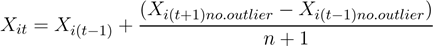
Isolated outliers were replaced by the average of the two immediately adjacent observations. However, if the outlier was the first or the last observation of the unit value, we replaced them by the trend of the closest observations. Occasionally, the outlier presented a rebound effect where the disruptive behavior was found in two consecutive periods. In these cases, both observations were replaced by the average of the variation between the non-outlier adjacent observations plus the value of the immediately preceding observation, as see in the following formula:
 (1)
(1)
where n = amount of adjacent outliers, X i,t = outlier in good i in time t.
Finally, a sequence of outliers (that we called step) were found in some unit values that are related to composition effects (Silver, 2007). The first observation of the step was replaced by the trend of the immediately previous observations and, for the rest of the sequence, their own variation was preserved. Therefore, only one observation is modified (the first one of the step) but the original behavior of the series is retained (see the example in Figure 1).
Source: own elaboration based on INDEC. Note: ISIC code 2699. Base year 2010 = 100.
Figure 1 Manufacture of other nonmetallic mineral products n.e.c.
As mentioned before, the sample selection of each sector had also a threshold on its homogeneity. When a certain unit value presented great volatility, we calculated the variation coefficient (VC) to define whether the high-volatility product should be dropped or replaced (Mendez, 2007; Garavito et al., 2014; INDEC, 1996). The threshold was defined ad hoc in the 4-digit sector by taking one or several reference products that showed a good performance. If the VC was strikingly high (more than the double of the reference VC), we replaced the product with a less volatile substitute or dropped it if there was no good substitute.
On the other hand, some products had a particularly high share in the 4-digits ISIC sector during the base period that may lead to a low representativeness in the rest of the years. This product could be a share outlier, i.e. a good significantly traded only in the base year. However, these cases are rare purchases or sales that do not represent the usual behavior of the unit value. Hence, we decided to analyze the volatility of their unit value and the degree of homogeneity comparing it with other products. If this product overcomes these tests, it remains in the sample and other items were included to gain representativeness in the years where it is scarce. If it does not overcome the tests, we replace it with some products that meet the criteria, at the expense of lower representativeness in the base year but gaining it in the rest of the period.
After the outliers’ detection and correction, we calculated the price indexes following the methodology of Gaulier et al. (2008). They were built according to the arithmetic formulas of Laspeyres, Paasche and Fisher, being this last one the geometric mean of the previous two. We chose these indexes because the benchmark statistics (from INDEC and Brazil) follow these formulas. However, a wide range of other indexes could be calculated (Laspeyres, Paasche, Fisher and Törnqvist; arithmetic and geometric, fixed base or chained) as well. We chose 2010 as a base year because it was a relatively stable period in which Gross Domestic Product (GDP) grew and prior to capital controls applied shortly afterwards in Argentina.
III. Results
A. Price indexes
In this subsection, the foreign trade price indexes are presented at the aggregate level and 2-digits ISIC sector. To assess the methodology, we compared our estimates with the aggregate indexes provided by INDEC and with Brazilian sectoral price indexes, in different aspects. On the one hand, Méndez (2007) argued that an index should have a VC of less than 50% to demonstrate that products that make up the sector are homogeneous. On the other hand, Gaulier et al. (2008) pointed out that the indexes with high correlation tend to show less discrepancy between them. We submitted our estimations to both testing criteria.
Table 1A and 2A in the Annexes contains the composition of imports and exports and the representativeness level in each sector, in detail. The most important 4-digits ISIC sectors (up to the 80% of total import value) include the following items: Motor vehicles and their parts, Communication devices, Chemical products, Fuels (oil and gas), Plastics and rubber, Iron and steel, Paper and paperboard, Machinery and tools, among others (Table 1A in Annexes). In relation to the representativeness level within each 4digits sector, only two sectors did not accumulate the 80% of their total value. Manufactures of precious metals and non-ferrous metals (ISIC code 2720) reached the 75% due to the high volatility of some of its items, meanwhile Manufactures of fertilizers and nitrogen compounds (ISIC code 2412) reached the 78% due to the discontinuity of the unit values. On the export side, only 17 sectors account for the 80% of the total value of exports (Table 2A in Annexes). This includes the following items: Production of oils and vegetable and animal fats, Cereals and other crops n.e.c., Manufactures of motor vehicles, among others. Unlike the basket of imports, the type of products are mostly primary commodities or some manufactures based on natural resources, with the only exception of the automobile industry. Likewise, the sample within each sector achieved more than the 80% of their total export value.
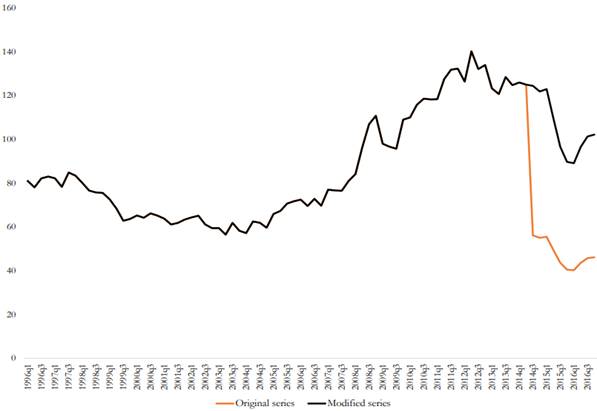
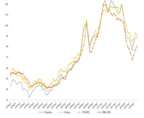
After assessing the sample representativeness level, we calculated the aggregate indexes according to the methodology described in the previous section. The Figures 2 and 3 contain our estimations, a series identified as INDEC, which corresponds to Argentine official estimates, and another one as Brazil, which corresponds to the indexes calculated by Fundação Centro de Estudos do Comércio Exterior (FUNCEX). The first one is a non-chained arithmetic Paasche index (INDEC, 1996), while the second one is a mixed arithmetic Fisher index (Pinheiro & Motta 1991; Guimarães et al., 1997; Markwald et al, 1998a and 1998b). Both statistical agencies collect information on prices through unit values estimates. There is a strong similarity between all the series, mainly in exports. In the case of imports, our indexes are very similar to the Brazilian ones, while the difference with INDEC is wider during the first years of the period. These results are the first evidence of the goodness of our methodology.
Source: own elaboration based on INDEC and IPEADATA-FUNCEX. Note: base year 2010 = 100.
Figure 2 Import Price Index
Source: own elaboration based on INDEC and IPEADATA-FUNCEX. Note: base year 2010 = 100.
Figure 3 Export Price Index
To verify the degree of correlation between these indexes, we built correlation coefficients6 (Gaulier et al., 2008). As can be seen in Table 1, the price indexes of imports and exports are highly correlated, which indicates that no outliers have been left in the sample.
Table 1 Correlation coefficients between the import and export price indexes
| Indexes | Imports | Exports | ||||||||
| Paasche | Laspeyres | Fisher | INDEC | BRAZIL | Paasche | Laspeyres | Fisher | INDEC | BRAZIL | |
| Paasche | 1.00 | 0.89 | 0.98 | 0.86 | 0.81 | 1.00 | 0.95 | 0.99 | 0.99 | 0.84 |
| Laspeyres | 1.00 | 0.97 | 0.81 | 0.83 | 1.00 | 0.99 | 0.96 | 0.87 | ||
| Fisher INDEC | 1.00 | 0.86 1.00 | 0.84 0.89 | 1.00 | 0.98 1.00 | 0.87 0.86 | ||||
| BRAZIL | 1.00 | 1.00 |
Source: own elaboration based on INDEC and IPEADATAFUNCEX.
On the other hand, when comparing our estimates with Argentine and Brazilian official indexes, we expected that the VC of our index does not duplicate those of the benchmarks. Regarding sectoral disaggregation, the criterion adopted by Méndez (2007) is followed, which considers that a VC less than or equal to 50% indicates that the products that make up the index are homogeneous.
At the general level, the INDEC index of imports has a volatility of 15% (well below the Brazilian one). As can be seen in Table 2, only the Paasche index doubles the variability of the INDEC. Regarding exports, the variability is lower and closer to the official indexes. Both INDEC and Brazil have indexes with the same variability (33%) and our estimated indexes have similar VC to the benchmarks.
Table 2 Variation coefficients of the aggregate import and export price indexes
| Imports | Exports | ||||||||
| Paasche | Laspeyres | Fisher | INDEC | BRAZIL | Paasche | Laspeyres | Fisher | INDEC | BRAZIL |
| 0.31 | 0.25 | 0.28 | 0.15 | 0.24 | 0.39 | 0.33 | 0.36 | 0.33 | 0.33 |
Source: own elaboration based on INDEC and IPEADATAFUNCEX.
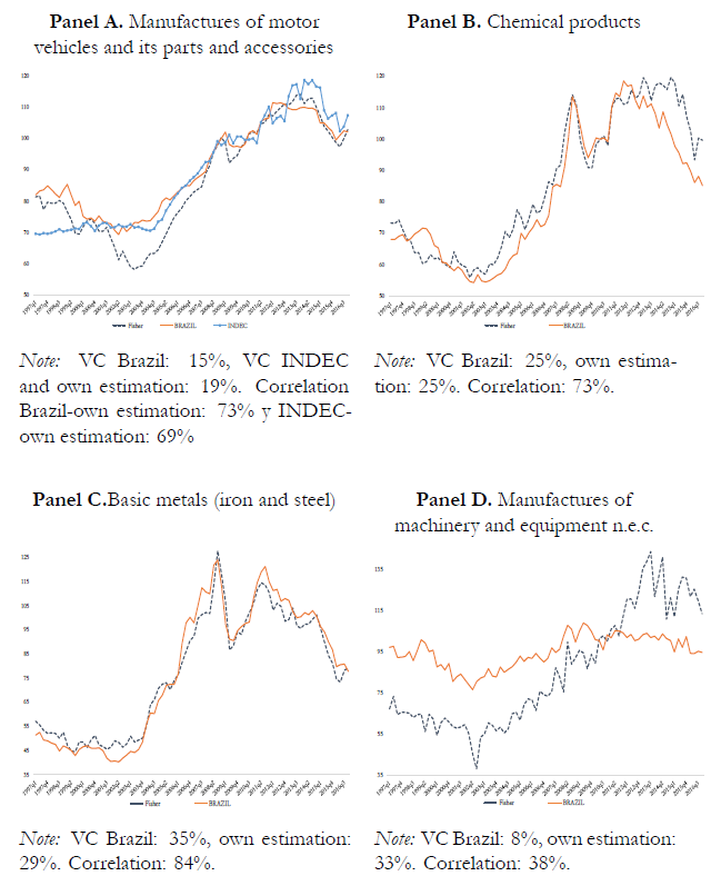
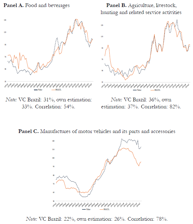
After confirming the accuracy of the methodology at the general level, the sectoral price indexes were constructed. In the case of imports, we estimated 87 price indexes (according to all types of indexes that were detailed in the methodology), of which the 86% have a VC less than 0.5 and none of them was higher than 1. Regarding exports, we estimated 83 indexes, of which the 88% showed a VC less than 0.5 and the remaining 12%, between 0.5 and 1. Thus, following Méndez (2007), we can claim that the products that compose the sample of these sectors are homogeneous.
Therefore, we selected some indexes to compare with Brazilian data (Figures 4 and 5). The chosen sectors represent the 50% of the total import and export value in the base year. The following graphs show the similarity and accuracy of our estimates, which allows us to continue, in the next subsection, to the volume indexes estimation.
Source: own elaboration based on INDEC and IPEADATA-FUNCEX. Note: base year 2010 = 100.
Figure 4 Import price indexes by sector
B. Quantity indexes
We calculated volume indexes by deflating import and export values by the price indexes estimated in the previous subsection. As can be observed in Figures 6 and 7, our aggregate volume indexes are very similar to those published by the INDEC, hence we can claim that the sectoral indexes are reliable. In relation to aggregate volumes’ evolution, imports show higher volatility than exports, which would be due to the greater fluctuations in Argentine GDP compared to those of its main trade partners.
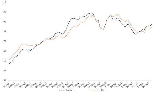
Source: own elaboration based on INDEC. Note: VC INDEC: 14%, own estimation: 16%. Correlation: 90%. Base year 2010=100, fourquarters moving average.
Figure 6 Aggregate export quantity index
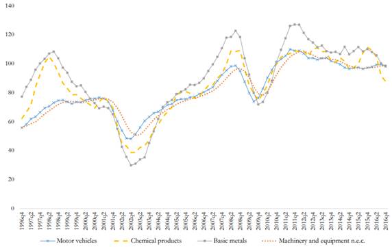
Hence, in Figure 8, we plot the quantity indexes of the most representative sectors of total imports. Motor vehicles, Chemical products, Basic metals and Machinery repeat the same pattern as in the aggregate level: a fall during the 1998-2002 recession, strong recovery between 2002-2008, new fall in 2008/2009, and stagnation with a downward trend since then.
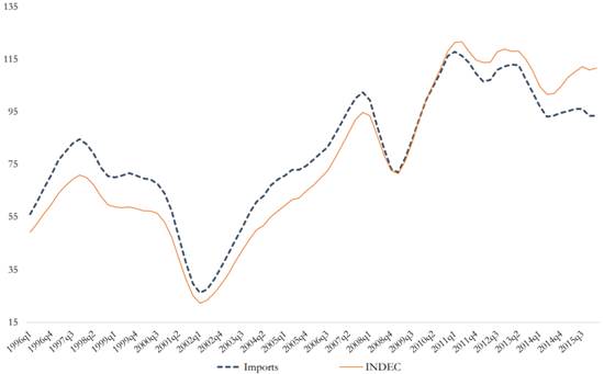
Source: own elaboration based on INDEC. Note: VC INDEC: 37%, own estimation: 28%. Correlation: 99%. Base year 2010=100, fourquarters moving average.
Figure 7 Aggregate import quantity index
Figure 9 shows the evolution of sectoral real exports. The Automobile industry is highly correlated with imports, which reveals the importance of the trade and production strategies implemented by firms that operates in Argentina and Brazil. On the other hand, Food and beverages show a growing trend over time, although it has been stopped by a recent stagnation. Finally, real exports of the agricultural products are less volatile during the whole period.
C. An empirical application: contribution by industry to foreign trade growth in Argentina (1996 -2016)
In this last section, we took advantage of our volume estimates to analyze the contribution of the main economic sectors in the growth rate of the real exports and imports during 1996-2016.
As shown in Table 3, the real exports grew at an annual average rate of 2.3% for the whole period. This is mainly explained by the agricultural products and manufactures based on agricultural resources (such as Food and Beverages), which showed an average annual growth rate of 4% and have a high initial share that increased towards the end of the period. On the other hand, Oil and natural gas extraction activity made an important negative contribution not only because of the average fall of 9% per year, but also because of its high initial share. In short, during the period 1996-2016, the export basket was concentrated in primary products and their manufactures, to the detriment of fuels and energy.
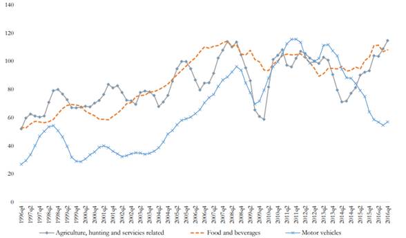
Source: own elaboration based on INDEC. Note: base year 2010 = 100, fourquarters moving average
Figure 9 Export quantity indexes by sector
Yet this period was not free of oscillations. Between 1996 and 2007, exports grew, almost uninterruptedly, for 12 years (there were only slight drops in 1999 and 2004). During these years, almost all sectors increased their exports, especially Motor vehicles and their parts, but with the exception of Oil and gas extraction activities. In 2008 and 2009, this growth was interrupted by subprime crisis and exports in real terms fell by an average of 7% per year. This was caused mainly by agricultural products due not only to the international crisis, but also to a domestic conflict between the government and the agricultural producers. In 2010 and 2011, the external trade improved, which was mainly driven by the agricultural and automobile industries, although in some extent compensated by Oil and gas. Then, in all sectors, a long fall averaged 6% per year until 2014. Finally, a slight recovery began in 2015, placing real exports at similar levels to 2005. In short, real exports have been stagnant for many years and all sectors seem to be related to the main trade partners’ business cycle, apart from oil and gas that shows an inverse relationship with the domestic business cycle.
Table 3 Evolution of real exports in Argentina by sector (19962016)
| Total | Sample | Beverages and food products | Agriculture, livestock, hunting and related service activities | Motor vehicles and their parts | Extraction of crude oil and natural gas | Rest | |
|---|---|---|---|---|---|---|---|
| Share in 1996 | 100% | 74% | 28% | 16% | 6% | 24% | 26% |
| Average growth rate in 199607 | 5.6% | 4.7% | 7.8% | 7.1% | 11.1% | 12.9% | 7.8% |
| Contribution to growth in 199607 | 1 | 0.59 | 0.44 | 0.22 | 0.16 | 0.23 | 0.41 |
| Share in 2007 | 100% | 68% | 35% | 19% | 10% | 3% | 32% |
| Average growth rate in 200709 | 6.9% | 8.7% | 6.3% | 25.1% | 8.6% | 43.5% | 3.3% |
| Contribution to growth in 200709 | 1 | 0.84 | 0.32 | 0.62 | 0.13 | 0.23 | 0.16 |
| Share in 2009 | 100% | 65% | 36% | 12% | 10% | 7% | 35% |
| Average growth rate in 200911 | 6.6% | 9.4% | 3.0% | 29.9% | 27.1% | 35.6% | 1.4% |
| Contribution to growth in 200911 | 1 | 0.93 | 0.16 | 0.62 | 0.44 | 0.29 | 0.07 |
| Share in 2011 | 100% | 68% | 33% | 18% | 14% | 2% | 32% |
| Average growth rate in 201114 | 6.0% | 6.1% | 3.5% | 8.8% | 8.9% | 8.1% | 5.8% |
| Contribution to growth in 201114 | 1 | 0.69 | 0.20 | 0.26 | 0.20 | 0.03 | 0.31 |
| Share in 2014 | 100% | 68% | 36% | 17% | 13% | 2% | 32% |
| Average growth rate in 201416 | 3.4% | 6.2% | 7.2% | 21.2% | 20.5% | 3.6% | 2.9% |
| Contribution to growth in 201416 | 1 | 1.27 | 0.78 | 1.14 | 0.69 | 0.02 | 0.27 |
| Share in 2016 | 100% | 72% | 39% | 23% | 8% | 2% | 28% |
| Average growth rate in 199616 | 2.3% | 2.2% | 4.0% | 4.1% | 3.6% | 8.9% | 2.8% |
| Contribution to growth in 199616 | 1 | 0.679 | 0.58 | 0.34 | 0.10 | 0.35 | 0.321 |
Source: own elaboration based on INDEC.
On the other hand, the import volumes showed an average annual growth rate of 2% for the whole period, somewhat lower than the export volumes (Table 4). This growth was explained in more than a half by the behavior of the Manufactures of motor vehicles and Chemical products. Due to the domestic business cycle, import volumes are more volatile than the export ones and have many more reversal points to the trend. The most significant fall took place between 1998 and 2002, when all sectors showed a significant decline (although by different magnitudes) because of the domestic economic crisis. The subsequent recovery took place up to 2008, when all sectors (except gas and oil) showed average annual rates very similar to the previous fall, but obviously, with the inverse sign and during a longer period. In 2009, the growth rate was interrupted by the transmission of the international economic crisis. All sectors were affected, except for oil and gas extraction, again. In 2010 and 2011, real import recovered, although in different magnitudes among sectors. Then, from 2012 until the end of the period (2016), real import decreased, in general terms, due to domestic economic stagnation, although led by machinery (vehicles, computers, TV, communication, electrical appliances, etc.) and with the exception of oil and gas. In short, the composition of the import basket has remained relatively stable, except for the growth of Motor vehicles and Chemical sectors and the decline of the Machinery of office, communication, radio and TV.
To sum up, import and export quantities, in both aggregate and sectoral levels, are closely related to the Argentine and its trade partners GDP growth rate, respectively. In fact, imports from all sectors fall between 1998 and 2002, due to the recession and subsequent economic crisis, and between 2008 and 2009 because of the international crisis on the domestic economy. The same happens for real export in all sectors during the last period. To know the effect of GDP and other variables, such as the exchange rate, on foreign trade, a specific study about elasticities should be made. Yet, this was not possible before this article because of the lack of price and quantity indexes at a deeper disaggregate level. Indeed, this article seeks to fill this gap in the statistics system of Argentina.
Table 4 Evolution of real imports in Argentina by sector (1996-2016)
| TOTAL | Sample | Motor vehicles and their parts | Chemical products | Basic Metals | Machinery and equipment n.e.c. | Extraction of crude oil and natural gas | Office, accounting and computing machinery | Electrical machinery and equipment n.e.c. | Radio, television and communications equipment and apparatus | Rest | |
|---|---|---|---|---|---|---|---|---|---|---|---|
| Share in 1996 | 100% | 67% | 11% | 15% | 4% | 15% | 7% | 6% | 5% | 5% | 33% |
| Average growth rate in 1996-98 | 17.3% | 18.6% | 31.1% | 18.0% | 22.9% | 13.7% | -35.1% | 38.4% | 22.6% | 27.7% | 14.5% |
| Contribution to growth in 1996-98 | 1 | 0.73 | 0.22 | 0.15 | 0.06 | 0.12 | -0.10 | 0.14 | 0.06 | 0.08 | 0.27 |
| Share in 1998 | 100% | 69% | 14% | 15% | 5% | 14% | 2% | 8% | 5% | 6% | 31% |
| Average growth rate in 1998-02 | -23.7% | -25.5% | -33.9% | -9.5% | -18.7% | -30.9% | -27.8% | -40.7% | -29.1% | -47.6% | -20.1% |
| Contribution to growth in 1998-02 | 1 | 0.72 | 0.17 | 0.07 | 0.04 | 0.17 | 0.02 | 0.11 | 0.06 | 0.08 | 0.28 |
| Share in 2002 | 100% | 63% | 8% | 29% | 6% | 10% | 2% | 3% | 4% | 1% | 37% |
| Average growth rate in 2002-08 | 23.8% | 25.5% | 40.4% | 13.5% | 19.4% | 30.9% | 5.8% | 33.0% | 27.4% | 57.4% | 20.7% |
| Contribution to growth in 2002-08 | 1 | 0.70 | 0.21 | 0.13 | 0.04 | 0.15 | 0.00 | 0.05 | 0.05 | 0.07 | 0.30 |
| Share in 2008 | 100% | 68% | 17% | 17% | 5% | 13% | 1% | 5% | 4% | 5% | 32% |
| Average growth rate in 2008-09 | -28.4% | -27.7% | -32.7% | -19.8% | -34.3% | -37.4% | 80.6% | -20.3% | -23.2% | -29.7% | -29.8% |
| Contribution to growth in 2008-09 | 1 | 0.66 | 0.20 | 0.12 | 0.06 | 0.18 | -0.02 | 0.03 | 0.04 | 0.06 | 0.34 |
| Share in 2009 | 100% | 69% | 16% | 19% | 5% | 12% | 2% | 5% | 5% | 5% | 31% |
| Average growth rate in 2009-11 | 26.9% | 28.8% | 42.4% | 19.6% | 23.2% | 32.6% | 58.6% | 11.2% | 35.4% | 12.8% | 22.7% |
| Contribution to growth in 2009-11 | 1 | 0.74 | 0.27 | 0.14 | 0.04 | 0.15 | 0.04 | 0.02 | 0.06 | 0.02 | 0.26 |
| Share in 2011 | 100% | 71% | 20% | 17% | 4% | 13% | 2% | 4% | 5% | 4% | 29% |
| Average growth rate in 2011-16 | -3.6% | -3.9% | -4.4% | -2.1% | -4.5% | -4.6% | 11.4% | -11.6% | -5.0% | -12.0% | -2.8% |
| Contribution to growth in 2011-16 | 1 | 0.76 | 0.25 | 0.11 | 0.05 | 0.16 | -0.11 | 0.11 | 0.07 | 0.12 | 0.24 |
| Share in 2016 | 100% | 69% | 19% | 19% | 4% | 12% | 5% | 3% | 5% | 3% | 31% |
| Average growth rate in 1996-16 | 2.4% | 2.6% | 5.1% | 3.7% | 2.1% | 1.3% | 1.1% | 2.0% | -1.8% | 2.9% | -0.6% |
| Contribution to growth in 1996-16 | 1 | 0.73 | 0.32 | 0.25 | 0.04 | 0.07 | 0.03 | -0.03 | 0.06 | -0.01 | 0.27 |
Source: own elaboration based on INDEC.
C. Final remarks
Currently, Argentina does not have a sufficiently complete and developed system of sectoral statistical data on foreign trade. In fact, INDEC provides price and volume statistics but only for total exports and imports and disaggregated by main classification of goods and economic uses, respectively. On the other hand, the INDEC’s foreign trade consultation system provides a large database, but only values and weight data are available, which are not like trade quantities, especially in differentiated goods. Thus, Argentina does not possess elemental foreign trade statistics by economic activities, such as prices and quantities.
In order to solve this limitation, we presented a methodology to calculate the import and export price indexes at the aggregate level and by 2-digits sectors of the ISIC classification. Providing this deeper disaggregation is very important because it allows us to use the indexes as deflators of values and thus to estimate import and export volumes by sector. In addition, the disaggregation that this work proposes, unlike that provided by the INDEC, has the same classification for export and import, so comparisons between trade flows could be made. Besides, it is based on an international classification, so it allows comparison with other countries. Finally, the same sectoral classification is used in data about other variables, such as value-added and employment, allowing more comprehensive studies to be carried out on different aspects of the economy.
Undoubtedly, the most challenging activity is the identification and treatment of outliers. The literature review in this matter is wide but, as we were working with time series samples in a broad period, we decided to follow the criterion based on the average price variation with an acceptance interval determined by the standard deviations of each product.
Once we obtain the estimated indexes, we compare them with the data provided by INDEC (aggregate indexes) and Brazil (indexes by economic sector) in order to test the accuracy of our methodology. Our estimations turned out to be reliable because, in addition to the good sample representativeness in all sectors, the correlation coefficients of the aggregate indexes were high, and they showed a variation coefficient quite like the domestic and international benchmarks. In this way, we can state that the methodology adopted was accurate and showed robustness when comparing it with Argentine and Brazilian official indexes.
Likewise, import and export price indexes by sector allow us to obtain the respective quantity indexes for Argentina, which showed, again, a high correlation with the INDEC estimates at the aggregate levels. Thus, we analyzed the contribution by economic activity to foreign trade growth during 1996-2016 by means of the estimated volume indexes.
To sum up, this article aims to contribute to the Argentine statistical system in a sensitive field such as foreign trade and economic sectors’ performance. From these data, studies about foreign trade, employment, growth and macroeconomics in general are substantially expanded. The contribution of this article is not only about providing the indexes but, especially, about showing our methodology. This could be replicated to estimate price and quantity indexes at an even deeper disaggregation, as well as for other countries that do not have this type of information available.