English (pdf)
 Article in xml format
 Article references
 Send this article by e-mail
 Cited by SciELO
  Cited by Google
  Similars in
SciELO
Similars in
SciELO  Similars in Google
 Permalink
Introduction
Modern economies are characterized by the co-existence of different forms of institutions, market structures, and a broad range of households with various endogenous changes in capital and knowledge. Combinations of these forms vary over time. It is important for dynamic economic theory to structurally explain the complexity. Different microeconomic theories study efficiencies and equilibrium of different market structures in varied economic institutions (e.g., Nikaido, 1975; Mas-Colell, et al. 1995; Brakman & Heijdra, 2004; Wang, 2012; Behrens & Murata, 2007, 2009; and Parenti, et al. 2017). Nevertheless, most of these studies are conducted with partial analytical frameworks. This study attempts to make a theoretical contribution to modelling economic growth with perfectly competitive as well as imperfectly competitive market structures in a general dynamic analytical framework. We integrate a basic model in neoclassical growth theory with a basic model in Stackelberg-Nash equilibrium theory. This study is based on a few well- established economic theories in economics literature. We frame the model on the basis of the Solow-Uzawa two-sector growth model. We consider a case in which the consumer goods sector in the Uzawa two-sector model is characterized by Stackelberg competition, rather than perfect competition as it is in the Uzawa model.
The purpose of this study is to make a contribution to economic growth theory by introducing a homogenous product market with Stackelberg competition to neoclassical growth theory. It attempts to make neoclassical economic growth theory more realistic in modelling the complexity of economic growth and development with different types of market structures. The Stackelberg model is one of the important strategic models in economics. It was designed by Heinrich Von Stackelberg in 1934. The model describes a leadership which allows the firm that dominates the market to decide its price first and in which follower firms subsequently make decisions to maximize profits. There are a number of works related to Stackelberg model with different adjustments for costs and capacities (e.g., Okuguchi, 1976, 1979; Howroyd & Rickard, 1981; Shapiro, 1989; Zhang and Zhang, 1996; Schoonbeek, 1997; Geraskin, 2017; Gong & Zhou, 2018; Prokop and Karbowski, 2018). In our study, we consider that a homogenous product market is characterized by a Stackelburg duopoly with one leader and one follower. The leader first decides the quantity of goods to be sold. The follower observes the leader’s decision and sets up its production quantity accordingly.
We construct an economy with two production sectors which are mainly framed in neoclassical growth theory. We deviate from the traditional Solow-Uzawa two-sector growth model only in one sector’s market structure. Neoclassical growth theory is mainly concerned with growth with endogenous saving. Capital accumulation is the economic mechanism of growth. It is one of the main modelling frameworks of economic growth and development with physical capital accumulation built upon microeconomic foundation (e.g., Solow, 1956; Uzawa, 1961; Burmeister & Dobell 1970; Azariadis, 1993; Barro & Sala-i-Martin, 1995; Jensen and Larsen, 2005; Ben-David & Loewy, 2003, and Zhang, 2008, 2020). Nevertheless, almost all models in the literature of neoclassical growth economic theory are developed for economies with perfectly competitive markets. As discussed extensively in Zhang (2005), neoclassical economic theory fails integrate different microeconomic theories partly due to analytical difficulties. Zhang (1993, 2005) applies an alternative approach to modelling household behavior. This approach has been applied to different economic problems. This study is another application of the approach to deal with a complicated issue in economic theory; how Stackelberg competition can be taken into account in neoclassical growth theory. It should be noted that new economic theory represents at attempt to introduce imperfect competition to macroeconomics (e.g., Dixit & Stiglitz, 1977; Krugman, 1979; Romer, 1990; Benassy, 1996; Nocco, et al., 2017). But new economic growth fails to include proper mechanisms of endogenous physical capital and wealth accumulation as a key growth factor. Zhang (2018) attempts to integrate new growth theory and neoclassical growth theory. Nevertheless, these studies in new growth theory do not consider Stackelberg competition theory in formal growth theory. This study introduces the Stackelberg duopoly model to neoclassical growth theory with capital accumulation. The rest of the paper is organized as follows. Section 2 builds a growth model of endogenous capital accumulation with perfect competition and Stackelberg competition. Section 3 studies the model’s analytical properties and identifies the existence of an equilibrium point. Section 4 carries out a comparative static analysis of a few parameters. Section 5 compares the economic performances of the traditional two-sector growth model and the model with Stackelberg competition. Section 6 concludes the study.
I. The growth model with Stackelberg competition
The basic contribution of this study is to introduce Stackelberg competition into the Solow-Uzawa neoclassical growth model with Zhang’s concept of disposable income and utility. For simplicity, we deal with duopoly. It is straightforward to generalize the model for any number of followers in Stackelberg competition. Most of the models are basically the same as the Solow-Uzawa neoclassical growth model, except for when it comes to modelling behavior of the household and behavior of duopoly. In our economy there are two kinds of goods and services-final goods and one duopoly product. In our model all markets for input factors are perfectly competitive. The final goods sector produces capital goods, which is the same as in the Solow model. It is invested and consumed. The final goods sector is the same as the one in the Solow model in which all markets are perfectly competitive. We follow the Uzawa two-sector modelling economic structure but assume that the consumer goods sector in the Uzawa model is composed of two firms and is characterized by Stackelberg competition. The duopoly product is solely consumed by consumers. The final goods sector and duopolists use capital and labor as inputs in producing final goods and duopoly products. In perfect markets (homogenous) firms have zero profit, while duopoly might have positive profits. For simplicity of analysis, profits are equally shared among the homogenous households. There is no free entry in duopoly products. The final goods are chosen to serve as a medium of exchange and are used as numeraire. We assume that capital depreciates at a constant exponential rate δ k .
A. The production of final product
We use F i (t), K i (t) and N i (t) to represent, respectively, output of the final goods sector, capital input and labor input. The production function of final goods is as follows:
 (1)
(1)
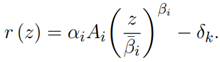
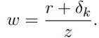
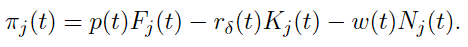
where A i , α i , and β i are parameters. We denote the wage rate and the interest rate with w(t) and r(t) interest rate. The profit of the final goods sector is:
π i (t) = F i (t) − (r(t) + δ k ) K i (t) − w(t)N i (t).
The following marginal conditions imply:
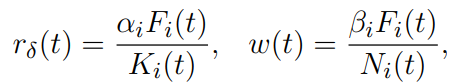 (2)
(2)
where rδ(t) ≡ r(t) + δk.
B. Consumer behaviors and wealth dynamics
This study applies the approach to modeling behavior of households proposed by Zhang (1993, 2005). Let
 stand for wealth of the representative household. We have
 where K(t) is the total capital. We assume that the profit is equally shared among households. It should be noted that in new growth theory profit is often assumed to be invested in innovation. This study neglects issues related to human capital, research, and knowledge creation. A more general approach should specify different possible distributions of profits among firms, households, and governments (for instance, in the form of taxation). Let h stand for human capital. We use π
j
(t) to stand for duopolist j
′
s profit. The current income of the representative household is:
where K(t) is the total capital. We assume that the profit is equally shared among households. It should be noted that in new growth theory profit is often assumed to be invested in innovation. This study neglects issues related to human capital, research, and knowledge creation. A more general approach should specify different possible distributions of profits among firms, households, and governments (for instance, in the form of taxation). Let h stand for human capital. We use π
j
(t) to stand for duopolist j
′
s profit. The current income of the representative household is:
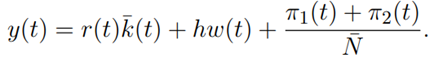 (3)
(3)
The household disposable income yˆ(t) is the sum of the current disposable income and the value of wealth as follows:
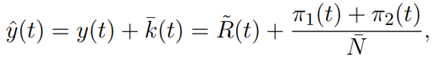 (4)
(4)
where

The representative household distributes the total available budget between consumption of monopoly product c j (t), and consumption of final goods c i (t), and savings s(t). The budget constraint is:
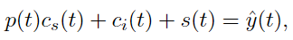 (5)
(5)
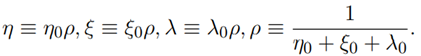
where p(t) is the price of consumer goods. We assume that utility level U (t) is dependent on c s (t), c i (t), and s(t) as follows:

where λ 0 is called the propensity to save. We solve the optimal problem as follows:
 (6)
(6)
Where
We see that the behavior of the household is determined once we solve p(t) and yˆ(t).
C. Wealth accumulation
According to the definition of s(t), the change in the household’s wealth is given by:
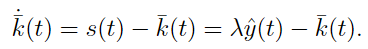 (7)
(7)
This equation implies that the change in wealth is equal to saving minus dissaving.
D. Equilibrium for the duopoly industry product
We use F j (t) to stand for the output of duopolist j. The equilibrium condition for duopoly product is given by:
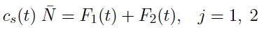 (8)
(8)
E. The behavior of the leader
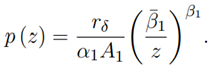
We now model the behavior of the leader. From (8) and (6) the demand function for the duopoly is given by:
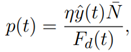 (9)
(9)
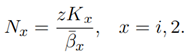
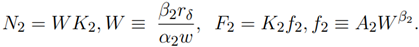
where F d (t) ≡ F1(t) + F2(t). We use Fj (t), K j (t), and N j (t) to represent respectively the output of duopolist j, its capital input, and labor input. We specify the production functions of the follower and leader as follows:
 (10)
(10)
where A j , α j and β j are parameters. The profit of duopolist j is
 (11)
(11)
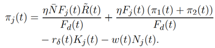 (12)
(12)
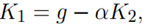
Add the two equations in (13)
 (13)
(13)
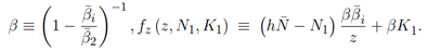
where
K d (t) ≡ K 1(t) + K 2(t), N d (t) ≡ N 1(t) + N 2(t)
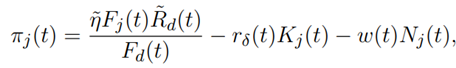 (14)
(14)
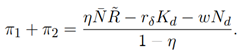
where η˜ = η/ (1 − η) and
R˜d(t) ≡ N¯ R˜(t) − r δ (t)K d (t) − w(t)N d (t).
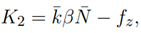
We assume that the duopoly industry is characterized by Stackelberg game dynamics, the leader is denoted with subscript 1 and the follower with subscript 2. We omit time in expressions when describing the behavior of the follower and the leader.
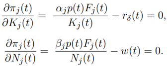
F. Behavior of the follower
The follower maximizes its profit with the leader’s output as given. The marginal conditions for the follower are:
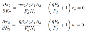 (15)
(15)
Divide the first equation by the second in (15)
 (16)
(16)
By (16) and the first equation in (15)
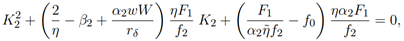 (17)
(17)
where we use F 2 = f 2 K 2 and
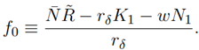
The follower’s optimal behavior is thus given by (17) and (16) as a function of the leader’s behavior as follows: K2∗ (K 1 , N 1) and N2∗ (K 1 , N 1).
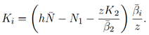
G. Behavior of the leader
From (14), we see that the leader’s profit is now given by:
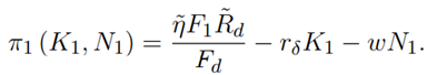 (18)
(18)
The leader maximizes its profit with K2∗ (K 1 , N 1) and N2∗ (K 1 , N 1) given as functions of its own behavior. The marginal conditions for the leader are:
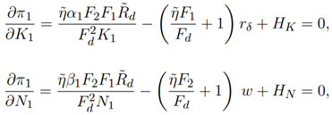 (19)
(19)
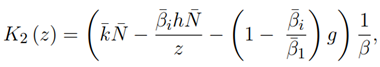
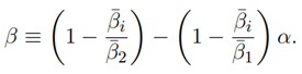
where
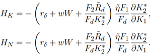
By (20) the leader’s behavior is determined. We determine the behavior of the follower by (18) as functions of the wage rate, the interest rate, wealth, and the other duopolist’s output and input factors. Each duopolist’s output and profit. The price of the duopoly product is given by (9).
H. Demand and supply of final goods
Change in capital stock equal to the output of the final goods sector minus the depreciation of capital stock and total consumption. We have the physical capital accumulation equation as follows:
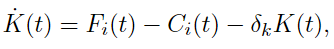 (20)
(20)
Where C i (t) = c i (t)N¯ .
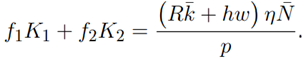
I. Labor and capital being fully utilized
The labor market clearing conditions are equal to labor supply and labor demand. We have:
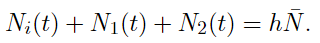 (21)
(21)
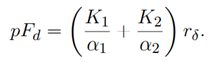
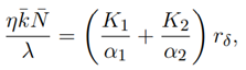
For capital markets we have:
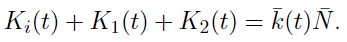 (22)
(22)
We built the model. The model is based on the Solow-Uzawa model, Stackelberg-Nash equilibrium model, and Zhang’s concept of disposable income and utility. We will now examine the model’s properties.
II. Equilibrium point
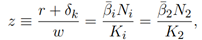
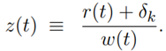
The previous section developed the Solow-Uzawa model by assuming that the consumer goods sector in the Uzawa two-sector model is characterized by Stackelberg-Nash equilibrium game dynamics. As it is difficult to explicitly analyze dynamic properties of the model, we provide a computational program to determine the movement of the economic system. We introduce
Lemma
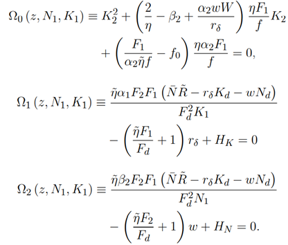
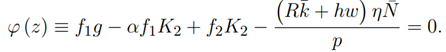
The dynamics of the economic system are given by the following differential equation:
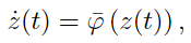 (23)
(23)
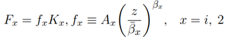
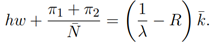
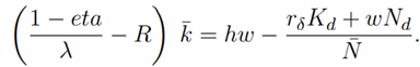
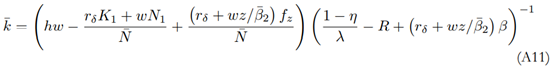
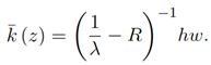
where function φ¯ (z(t)) is defined in the Appendix. All the other variables are explicitly given as functions of z(t) as follows: r(t) by (A2) → w(t) by (A3) → k¯(t) by (A11) → K(t) = k¯(t)N¯ → K 2(t) by (A7) → K i (t) by (A6) → N 2(t) by (A1) → N i (t) by (A1) → F i (t) and F 2(t) by (A4) → F 1(t) by (10) → R˜(t) by (4) → π j (t) by (14) → yˆ(t) by (4) → p(t) by (9) → c i (t), c j (t)
and s(t) by (6) → U (t) by the definition.
We now examine the economy’s behavior. It is difficult to give a general solution to the problem. In the rest of the paper, we are concerned with equilibrium as it is difficult to carry out genuine dynamic analysis. To determine the equilibrium values of the economic system we specify the rest of the parameters as follows:
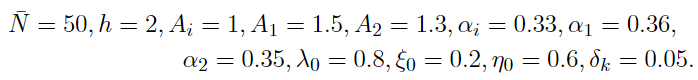 (24)
(24)
The population is 50 and human capital is 2. Although the specified values of the parameters are not referred to any given economy, we can get insights into the economic mechanism of growth by studying effects of different values of these parameters on the national economy. The simulation identifies an equilibrium point. The equilibrium values are as follows:
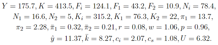 (25)
(25)
In (25), the national income and profit per unit of output π¯j are defined as:
We see that final goods sector has zero profit due to perfect competition and the leader and follower have positive profits due to market power. The leader has higher profit per output than the follower. We now study how the equilibrium structure is affected when parameters vary.
III. Comparative Static Analysis
The previous section showed growth equilibrium of the national economy with perfect competition in input factor and final goods markets and Stackelberg-Nash equilibrium in consumer goods market. We now examine how the national economy is affected when some exogenous conditions such as preference and technologies are changed. As the lemma provides a computational procedure to calibrate the model, it is straightforward for us to examine the effects of changes in any parameter on the equilibrium values of the economic system. We define a variable ∆¯ x to represent the percentage change rate in the variable x due to changes in the parameter value.
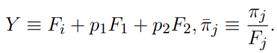
A. The leader’s total factor productivity is enhanced
We first study what happens to the economic system if the leader’s total factor productivity is enhanced as follows: A 1 = 1.5→1.55. The effects on the variables are listed in (26). The leader’s output has increased. The leader employs less labor force and more capital. The leader earns more profit, and its profit rate has increased. The follower produces less and employs less labor and capital inputs. The follower has less profit, and its profit rate is reduced. The final goods sector increases its output and employs more labor and capital inputs. The national output and capital are augmented. The wage rate rises, while the interest rate falls. The price of consumer goods falls. The household has more income and disposable income. The household consumes more final goods and consumer goods and has a higher utility level.
 (26)
(26)
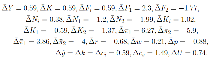
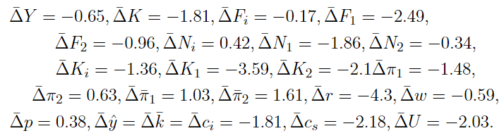
B. The follower’s total factor productivity is enhanced
We now examine what happens to the economic system if the follower’s total factor productivity is enhanced as follows: A 2 = 1.3→1.35. The effects on the variables are listed in (27). The follower produces more and employs more labor and capital inputs. The follower earns more profits and its profit rate is enhanced. The leader’s output is decreased. The leader employs less labor force and capital inputs. The leader earns less profit and its profit rate is decreased. The final goods sector reduces its output and employs less labor and capital inputs. The national output and capital are reduced. The wage rate and interest rate rise. The price of consumer goods falls. The household has less income and disposable income. The household consumes fewer final goods and consumer goods and lower higher utility level. It should be noted that in contrast to the case where the leader has higher total productivity, when the follower has higher total factor productivity, the national output is reduced. This occurs because the follower obtains more market share. As the follower’s total factor productivity is still lower the leader’s, the national output is reduced as more resources are shifted from the leader to the follower.
 (27)
(27)
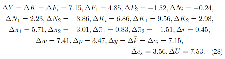
C. The final goods sector’s total factor productivity is enhanced
We now analyze what happens to the economic system if the final goods sector’s total factor productivity is enhanced as follows: A i = 1→1.05. The effects on the variables are listed in (28). The final goods sector increases its output. The sector employs less labor force and more capital input. The leader’s output is increased. The leader employs more labor force and capital inputs. The leader earns more profits, and its profit rate increases. The follower produces less and employs less labor but more capital inputs. The follower has lower profits, and its profit rate is reduced. The national output and capital are augmented. The wage rate and interest rate rise. The price of consumer goods is increased. The household has more income and disposable income. The household consumes more final goods and consumer goods and has higher utility level.
 (28)
(28)
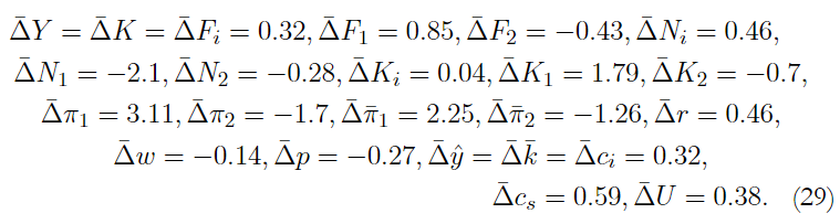
D. The leader’s output elasticity of capital is increased
We now study what happen to the economic system if the leader’s output elasticity of capital is increased as follows: α 1 = 0.36→0.37. The effects on the variables are listed in (29). The leader’s output is increased. The leader employs less labor force and more capital. The leader earns more profit and its profit rate is increased. The follower produces less and employs less labor and capital inputs. The follower has less profit and its profit rate is reduced. The final goods sector increases its output and employs more labor and capital inputs. The national output and capital are augmented. The wage rate falls, while the interest rate rises. The price of consumer goods falls. The household has more income and disposable income. The household consumes more final goods and consumer goods and has higher utility level.
 (29)
(29)
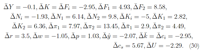
E. The propensity to consume consumer goods is enhanced
We now examine what happen to the economic system if the propensity to consume consumer goods is enhanced as follows: η 0 = 0.1→0.11. The effects on the variables are listed in (30). The final goods sector reduces its output. The sector employs less labor force and capital inputs. The leader’s output is increased. The leader employs more labor force and capital inputs. The leader earns more profits and its profit rate is increased. The follower produces more and employs more labor but more capital inputs. The follower has more profits and its profit rate is enhanced. The national output and capital are decreased. The wage rate falls, while the interest rate rises. The price of consumer goods is increased. The household has less income and disposable income. The household consumes fewer final goods but more consumer goods. The household has a lower utility level.
 (30)
(30)
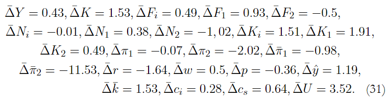
F. The propensity to save is enhanced
We now study what happens to the economic system if the propensity to save is enhanced as follows: λ 0 = 0.8→0.81. The effects on the variables are listed in (31). The final goods sector increases its output. The sector employs less labor force but more capital inputs. The leader’s output is increased. The leader employs more labor force and capital inputs. The leader earns less profits and its profit rate is reduced. The follower produces less and employs less labor force but more capital input. The follower earns less profits and its profit rate is decreased. The national output and capital are increased. The wage rate rises, while the interest rate falls. The price of consumer goods is decreased. The household has more income and disposable income. The household consumes more final goods and consumer goods. The household has a higher utility level.
 (31)
(31)
G. The depreciation rate of capital is increased
We now examine the effects of the following rise in the depreciation rate of capital: δ k = 0.05→0.055. The effects on the variables are listed in (32). The final goods sector reduces its output. The sector employs more labor force but less capital input. The leader’s output is decreased. The leader employs less labor force and capital inputs. The leader earns less profit, but its profit rate is increased. The follower produces less and employs less labor force and capital input. The follower earns more profits and its profit rate is increased. The national output and capital are decreased. The wage rate rises, while the interest rate falls. The price of consumer goods is decreased. The household has less income and disposable income. The household consumes fewer final goods and consumer goods. The household has a lower utility level.
 (32)
(32)
We also conducted analyses for changes in the population and human capital, which cause proportional changes in the real variables and no changes in prices.
IV. Comparing Growth with Stackelberg Competition and Perfect Competition
This section compares the dynamics of the model with Stackelberg competition and the two-sector model with perfect competition. When the system is perfectly competitive, firms take prices as given and equilibrium condition of demand supply determine price. We describe the growth model when the consumer goods market is perfectly competitive. A main difference is that profit is zero in perfect competition, i.e., π j (t) = 0. Profits and marginal conditions for the two firms are as follow, respectively
 (14’)
(14’)
 (15’)
(15’)
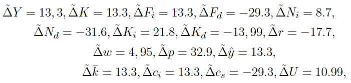
where equations (11)’ and (15)’ correspond to, respectively, (14) and (15). The equations in Section 2, except those related to the leader’s and follower’s profits and marginal conditions, also true for the perfectly competitive case. In Appendix A2, we provide a computational program to determine equilibrium of the competitive model. We calculate the equilibrium point of the perfectly competitive system under the same parameter values in (27). The result is listed in (36).
 (33)
(33)
in which

In the case of perfect competition firm 2 in the consumer goods sector produces nothing. In this case firm 1’s behavior represents the consumer goods sector’s behavior. From (33), we conclude that in Stackelberg competition the national output and national capital (and thus household wealth) are higher than in the perfectly competitive economy. In Stackelberg competition the final goods sector produces more and employs more labor and capital inputs, while the consumer goods sector produces less and employs less labor and capital inputs. The interest rate is lower, the wage rate is higher, and price of consumer goods is higher in Stackelberg competition. The household has more disposable income, consumes more final goods, consumes less consumer goods, and has higher level of utility in Stackelberg competition. We see that if the profits of the Stackelberg duopoly are equally distributed amongst the households, the household has higher welfare when the consumer goods market is characterized by Stackelberg competition, rather than by perfect competition.
Concluding remarks
This study introduced Stackelberg-Nash equilibrium to neoclassical growth theory with Zhang’s concept of disposable income and utility. The paper makes neoclassical economic growth theory more robust in modelling the complexity of market structures. It integrates neoclassical growth theory with one of the basic industrial structures developed in microeconomics. The model is based on a few well-established economic theories in the literature of economics. We framed the model within the Solow-Uzawa two-sector model. The economy is composed of two sectors. The final goods sector is the same as in the Solow one-sector growth model which is characterized by perfect competition. The consumer goods sector is the same as the consumer goods sector in the Uzawa model but is characterized by Stackelberg duopoly. The modelling of Stackelberg-Nash equilibrium is based on traditional Stackelberg game theory. We modelled household behavior with Zhang’s concept of disposable income and utility. This research integrated these theories in a comprehensive framework. It endogenously determines profits of duopoly which are equally distributed among the homogeneous population. We built the model and then identified the existence of an equilibrium point by simulation. We conducted comparative static analyses in some parameters. We also compared the economic performances of the traditional Uzawa model and the model with the Stackelberg-Nash equilibrium. We concluded that the imperfect competition increased national output, national wealth, and utility levels in comparison what is seen with perfect competition. As this is based on some simple cases of well-developed theories and each theory has its own complicated literature, it is not difficult to extend and generalize our model conceptually and analytically. We may take into account capacity constraints in modelling the Stackelberg game. It is important, for instance, to include location differentiation such as regional science and urban economics. It is straightforward to generalize the model by introducing more goods in to competitive markets and other forms of imperfection (e.g., Dixit and Stiglitz, 1977; Romer, 1990; Wang, 2012; and Zhang, 2018, 2020).