Inglés (pdf)
 Articulo en XML
 Referencias del artículo
 Enviar articulo por email
 Citado por SciELO
  Citado por Google
  Similares en
SciELO
Similares en
SciELO  Similares en Google
 Permalink
Introduction
Global wealth inequality decreased during the first eight decades of the XX century. An index like the top 1% personal wealth share shows a consistent downward trend from 1913 to around 1980, but in the 1980’s, the index rebounds and rises consistently in countries such as the United States, the United Kingdom, France, Russia, and China (Alvaredo et al., 2018). According to the same authors, wealth inequality increased in nearly all world regions in recent decades as did income inequality. Moreover, this rising trend does not show any sign of receding but of deepening: “if established trends in wealth inequality were to continue, the top 0.1% alone will own more wealth than the global middle class by 2050” (p. 198).
As Piketty (2014) and many others have shown, the reversion of the wealth concentration process is clearly related to the political environment. The first eight decades of the XX century were marked by the construction of different kinds of welfare states, whilst the strong reversion towards inequality is related to the partial dismantling of welfare states, the orientation towards labour market flexibilization, and the adoption of the Washington Consensus.
This paper, however, is not concerned about the explanation of economic inequality trends; it focuses instead on its welfare consequences and the economic policies to tackle the problem. In order to do that, I build on the model of Ortiz and Castillo (2020). In this model (hereafter, the original model), the concentration of capital ownership delivers three important economic features: 1) economic activity decreases, 2) income distribution systematically shifts in favour of capital, and 3) labour unemployment increases when the degree of capital ownership concentration surpasses a certain threshold. Thus, in this theoretical set up, capital ownership concentration systematically diminishes the population’s purchasing power.
How relevant are those characteristics in the world economy? The World Bank (n.d.) shows that economic growth deceleration is a consistent trend since the 1960’s. Figure 1 depicts the annual economic growth rate for high income countries from 1961 to 2019.
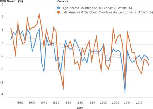
Source: World Bank (n.d.).
Figure 1 High Income Countries and Latin America: Annual Economic Growth (%)
It has been argued that this falling economic activity level is due to the global productivity slowdown. It may be, but it does not deny the possibility that systematic losses of the population’s purchasing power explain a significant part of the story.
With respect to the losses of labour remuneration as a fraction of income, there is also some empirical evidence. Taking into account the difficult issue of labour informality, the International Labour Organisation (ILO) has revealed a consistent decline of the labour income share in the global economy.
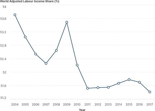
Figure 2 reveals that labour remuneration as a fraction of the world output is declining. The financial crisis of 2008-2009 reversed that trend temporarily because of the sudden contraction of global output. The analysis took into account the household surveys for 95 countries from 2004 to 2017 and showed that “the global labour income share is declining and countercyclical, similar patterns arise in the European Union and the United States” (ILO, 2019b, p. 39).
In the original model, the unemployment rate increases as capital ownership concentrates in fewer hands. This characteristic is not observed in the real world. The original model was too simple and did not include informal workers. Labour informality, however, remains pervasive around the world. According to ILO (2019b), high informality rates (well above 50%) persist in low- and middle-income countries; as a matter of fact, nowadays three out of five workers worldwide are informal, and they earn low wages.
Thus, a simple theoretical construction such as the original model replicates with some success some characteristic patterns of economic development in the last 60 years. The social effects of workers’ relative income losses, however, were ignored in the original analysis. This paper fills that gap by explicitly considering some government redistributive policies: the minimum wage rate, an unemployment insurance program, and the payment of a universal basic income. It goes without saying that the government plays an active role in these new analyses. The government has to enforce the minimum wage law and must collect taxes on income from capital to finance the unemployment insurance program and/or the universal basic income program.
The original model found that the price mechanism equilibrates the economic system for intermediate degrees of capital ownership concentration. When this concentration of wealth surpasses a certain threshold, the wage rate cannot fall any longer and it is fixed at the socially established minimum level. Political conditions and economic welfare considerations may induce the fixation of a minimum wage rate above the subsistence income. In any case, when the economy reaches the minimum wage rate, the price system breaks down as an economic device to clear the labour market and labour unemployment increases with the process of capital concentration.
The Original Model
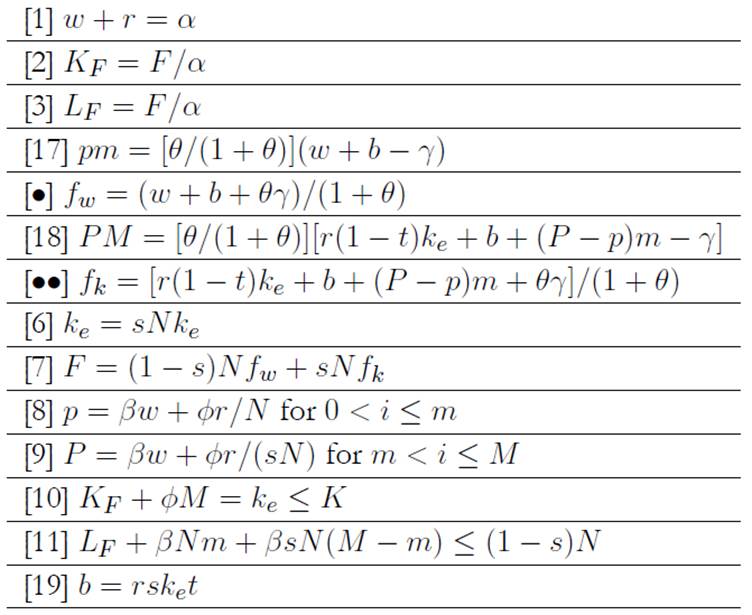
The model structure is briefly shown in Equation System 1.
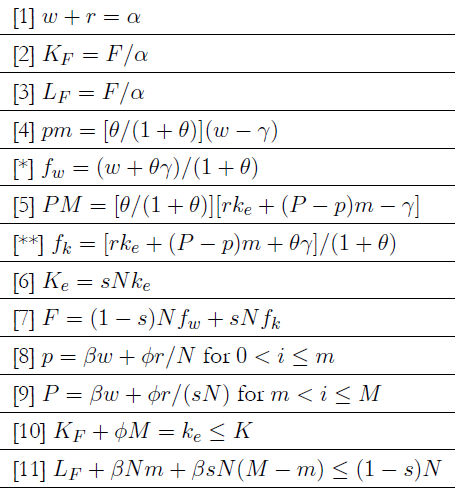
This market economy has capital and labour as factors of production. Two kinds of goods are produced: food and manufactures. The food technology is given by a Leontief production function: F /α = min (KF, LF), where F is the food production in the period of analysis, α is the sector’s multifactor productivity, and KF and LF are the amount of capital and labour used in this activity. The user cost of capital is denoted with r, and the wage rate is denoted with w. Food is taken as numeraire. Hence, Equation (1) is the sector’s factor price frontier in a competitive environment. And Equations (2) and (3) are the sector factors’ demands.
Capital and population, K and N, are given at any production period. Labour is homogeneously distributed among the N members of this economy (one unit per capita). It is also assumed that ownership of capital is homogeneously distributed among capitalists. They represent a fraction s of the population; thus, s becomes an inverse measurement of capital ownership concentration. No one can be a worker and a capitalist at the same time. Capital is inelastically supplied at non-negative prices; but labour is inelastically supplied for wage rates equal to or higher than the subsistence income, as it will be defined below.
Worker preferences are given by the following utility function: Z(fw, m) = ln(fw ─ γ) + θ ln (m), where fw is the amount of food consumed in the period of analysis by the typical worker, γ is the minimum amount of food that a person needs during the production period (the subsistence income), m is the diversification index of manufacturing goods for workers, and θ is a constant that measures the consumer bias towards manufacturing consumption. Given the typical worker budget restriction: fw + pm = w, where p is the price of the manufactured goods which are consumed by workers, Equations (4) and * denote the typical worker demands of food and manufactures.
For a typical capitalist the consumption problem is set as follows: maximize the utility function Z (fk, M) = ln (fk ─ γ) + θ ln (M) subject to the following budget restriction: fk + pm + P (M─m) = r Ke, where fk is the amount of food consumed in the period of analysis by the typical capitalist, M is the typical capitalist index of manufacturing consumption diversification, P is the common price of all those manufacturing goods which are demanded only by capitalists (the low-demand goods), the difference M m is the range of low-demand manufacturing goods, and Ke is the amount of effective capital per capitalist (notice that a typical capitalist consumes the same m manufacturing goods that a typical worker does plus some others). As in the case of high-demand goods, supply and demand of low-demand goods are assumed to be identical across these goods; that is why they all have the same price. The solution of this optimization problem yields the typical capitalist demand functions of manufactures and food, Equations (5) and (**), respectively.
A sensible equilibrium for this market economy must imply that the typical capitalist remuneration, rke, is higher than the wage, w. Capitalists have more freedom to choose. As they own the available capital, they can become entrepreneurs; but they may also give up being capitalists and become workers. On the other hand, the exclusion from capital ownership only gives the option of being a worker.
Effective aggregate capital demand is given by Equation (6), where ke is the fraction of total capital which is effectively used in economic activities. Aggregate food demand is given by Equation (7); the workers and capitalists’ food demands are added up.
Manufacturing goods are all produced with the following increasing returns to scale technology: a fixed investment of ϕ units of capital is needed to design a new manufacturing good, and β units of labour are required to produce one manufacturing good. Since market entry and exit are assumed to be free, prices should be set for all manufacturing goods such that profits are null. Hence, the equilibrium prices of high-demand manufacturing goods and low-demand manufacturing goods, p and P, should satisfy Equation (8) for high-demand manufacturing goods and Equation (9) for low-demand manufacturing goods.
Due to consumption rigidities, this economic system does not guarantee equilibrium in the factor markets. In any case, aggregate capital demand, ke, cannot exceed capital supply, K, which delivers inequality (Equation (10)). And aggregate labour demand cannot exceed labour supply, which delivers inequality (Equation (11)).
All parameters denoted with Greek letters are assumed to be constant. The population (N), the capital stock (K), and the population fraction of capitalists (s) are also given at any production period. Hence, the economic system has eleven unknown variables: w, r, F, KF, LF, p, P , m, M , ke and ke. With nine equations and two inequalities, the possibility of a general equilibrium exists if the slackness is suppressed (labour and capital markets clear).
As previously mentioned, in this model wealth concentration implies a lower aggregate purchasing power, which implies a falling GDP. Wealth concentration directly increases labour supply, and that, in turn, forces a lower labour remuneration so that a distributive shift in favour of capital takes place. This process continues until the labour remuneration hits its minimum level, which might be above the subsistence income. Further capital concentration comes at a cost of increasing labour unemployment. Since the unemployed are left incomeless, they drop from the markets and aggregate demand falls even quicker. If there is any social empathy, the government has to step in and do something. In such a case, two economic policies will be considered: 1) an insurance program to pay the basic consumption for the unemployed and 2) a universal basic income payment. Both policies are financed with taxation on capital returns.
A key feature of the original model is the explicit consideration of basic consumptions -a minimum level of food is required by every person, and manufacturing goods of lower index are preferred to manufacturing goods of higher index. Thus, food requirements are paramount, but there are also manufactured goods whose provision has to come first. In addition, preferences are satiable (none or just one unit of each manufacturing good is consumed per person). In that sense this model follows the treatment of consumer preferences that were considered by Murphy et al. (1989b).
The model which is developed here, however, is structurally much simpler: land as a productive factor is included in capital (there are no land rents to be considered), the distribution of capital ownership is assumed to be homogeneous among capitalists, and the utility function is also simpler. Hence, it is possible to find explicit numerical solutions. The model also considers productive diversification and increasing returns to scale in the manufacturing sector, as in the models of Murphy et al. (1989a). These authors model the economic development analysis of Adam Smith (1776/1981), which is based on the interaction between “division of labour” (productive diversification as the main engine of productivity gains driven by increasing returns to scale) and “extent of the market” (population purchasing power).
The models which are built in this paper are kept explicitly static, like the original one, in order to avoid the mathematical complexities of intertemporal choices. Finally, the assumption of non-homothetic preferences prevents the income and capital distribution to be neutral; with homothetic preferences, the structure of consumption is preserved regardless of the income level so that a single rich person with enough income may replace the consumption of many. This is, of course, absurd. As people get richer, the marginal utility of basic goods tends to decrease; and the consumption of most manufacturing goods usually stops after the first unit (no one sleeps in two beds at the same time). Instead, people diversify their consumption basket. That is why the capital ownership concentration process, which also concentrates income in the capitalists’ hands, leads to a lower aggregate purchasing power.
When the model is solved for explicit prices, it reveals that a minimum volume of population is required in order to have a manufacturing industrial sector. Given the fixed costs of these activities, a minimum aggregate demand is required for the economic system to operate without losses.1 Once this condition is fulfilled, the model solutions reveal that a minimum degree of capital ownership concentration is also required for the manufacturing activity to take off; very low capital concentration may yield an individual capitalist remuneration below the wage rate, so that the manufacturing activity collapses.2 For intermediate degrees of capital ownership concentration, the economic system may work with factor markets clearing; there are no unemployed resources, and there exists a unique set of price solutions for factors and goods that guarantees the general economic equilibrium. Everything changes, however, when the economic system reaches or surpasses some threshold level of capital ownership concentration. In this case, the wage remuneration ought to be fixed to a minimum level which may be equal or higher than the subsistence income. Labour unemployment appears, and the effective demand for capital exceeds actual supply so that capital is fully employed. In any case, the process of capital ownership concentration diminishes the population’s purchasing power and leads to a decreasing GDP.
An Unemployment Insurance Program
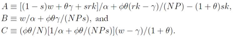
This section considers an unemployment insurance program within the economy analysed in the original model. For simplicity, it is assumed that an unemployed person gets a remuneration equivalent to the minimum food consumption per person (γ); this assumption means that the unemployed are excluded from manufacturing consumption. In this situation the economic system is modified as follows:
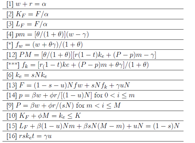
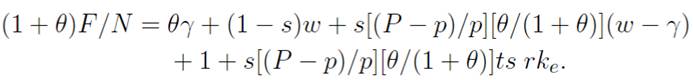
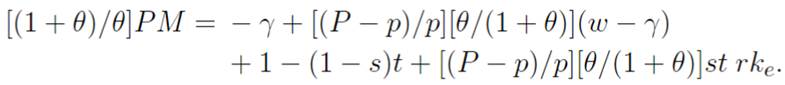
A key issue in this new economic system is that capitalists pay taxes on their returns. Being t the tax rate, the typical capitalist returns after taxes are given by r(1─t)ke. That explains why Equations (5) and (**) in Equation System 1 become Equations (12) and (***), the typical capitalist demand equations for manufacturing goods and food. Now, in this new set up, u is the labour unemployment rate calculated over the whole population (N). It is also assumed that the government pays an unemployment insurance that just covers the minimum food requirement. Hence, aggregate food demand, F, is modified in two ways: 1) with labour unemployment (u > 0), the fraction of workers (who demand food) is reduced from 1─s to 1─s─u and 2) food demand increases however with the government insurance program by γuN . These two changes explain why Equation (7) becomes Equation (13). Since the unemployed drop from the manufacturing sector demand, the average fixed cost of high-demand goods increases to ϕr/[(1─u)N ]; that explains the transformation of Equation (8) into Equation (14). Capital market equilibrium is unchanged, bearing in mind that effective capital demand is restricted to capital supply (Ke = K). The labour market however may be in disequilibrium because labour demand is shortened by the lower aggregate demand. Hence, labour demand from the agricultural sector (LF), plus labour demand from the high-demand manufacturing goods sector [β(1─u)Nm], plus labour demand from the low-demand manufacturing goods sector [βsN (M─m)], plus the unemployed (uN ) equals labour supply [(1─s)N ]. Finally, the long-run fiscal equilibrium imposes that tax collection on capital returns equals government spending r Ke t = γuN . Substitution of Equation (6) in the later condition yields equation (16).
The results reveal, as in the original model, that very low capital ownership concentration (high s) is not viable under a capitalist regime. For intermediate degrees of capital concentration, there exists a set of prices so that markets clear. Hence, if u = 0, the model collapses to the original model. Here, it is explicitly considered the case that where the degree of capital ownership concentration is high, the effective capital demand is too high (all capital is employed), the labour demand is too low (unemployment arises), the government fixes a minimum wage rate that might be above the subsistence income, and it pays the subsistence income to the unemployed as unemployment insurance. This difference between the minimum wage and the subsistence income ensures that everyone prefers to be a worker rather than an unemployed person. The minimum wage rate was proposed initially as politically determined, but the model will reveal that a minimum wage may be optimally chosen to minimize the unemployment rate; and this optimal minimum wage is above the income remuneration.
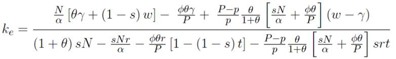
The mathematical solution of this new system under a high degree of capital ownership concentration is confined to Appendix 1. Just bear in mind that in those conditions the wage is fixed at the minimum level; effective capital demand, ke, exceeds capital supply, K so that Ke = K, and Ke = k.
The model is static. The population fraction of capitalists, s, is assumed to be given at any moment (see Column 1). Each row of Table 1 presents the model results for a given s at a given period. A process of capital ownership concentration might be considered by diminishing s continuously, as it is done along the first column in an exercise of comparative statics.
Table 1 The Model with Minimum Wage and Unemployment Insurance
| S (1) | W (2) | R (3) | T (4) | P (5) | P (6) | M (7) | M (8) | k e (9) | r(1- t)k e /w (10) | f w (11) | f k (12) | F (13) | KF = LF 14) | GDP (15) | U (16) |
|---|---|---|---|---|---|---|---|---|---|---|---|---|---|---|---|
| 0.24 | 1.33 | 0.67 | 0 | 1.76 | 1.83 | 0.20 | 0.21 | 2.08 | 1.04 | 0.98 | 1.02 | 59.2 | 29.6 | 80.8 | 0 |
| 0.23 | 1.25 | 0.75 | 0 | 1.66 | 1.74 | 0.20 | 0.28 | 2.17 | 1.29 | 0.93 | 1.15 | 58.9 | 29.4 | 80.3 | 0 |
| 0.22 | 1.17 | 0.83 | 0 | 1.55 | 1.65 | 0.19 | 0.36 | 2.27 | 1.60 | 0.89 | 1.30 | 58.5 | 29.3 | 79.7 | 0 |
| 0.21 | 1.09 | 0.91 | 0 | 1.45 | 1.57 | 0.18 | 0.46 | 2.38 | 1.97 | 0.84 | 1.46 | 58.2 | 29.1 | 79.0 | 0 |
| 0.20 | 1.01 | 0.99 | 0 | 1.35 | 1.48 | 0.16 | 0.58 | 2.50 | 2.45 | 0.79 | 1.64 | 57.7 | 28.8 | 78.2 | 0 |
| 0.19 | 0.92 | 1.08 | 0 | 1.23 | 1.39 | 0.15 | 0.73 | 2.63 | 3.08 | 0.74 | 1.85 | 57.1 | 28.5 | 77.1 | 0 |
| 0.18 | 0.82 | 1.18 | 0 | 1.10 | 1.28 | 0.12 | 0.94 | 2.78 | 4.02 | 0.68 | 2.10 | 56.2 | 28.1 | 75.7 | 0 |
| 0.17 | 0.66 | 1.34 | 0 | 0.91 | 1.12 | 0.08 | 1.32 | 2.94 | 5.94 | 0.59 | 2.47 | 54.7 | 27.4 | 73.1 | 0 |
| 0.16 | 0.6 | 1.4 | 0.012 | 0.83 | 1.07 | 0.05 | 1.53 | 3.13 | 7.21 | 0.56 | 2.69 | 53.9 | 26.9 | 71.6 | 0.017 |
| 0.15 | 0.6 | 1.4 | 0.027 | 0.83 | 1.09 | 0.05 | 1.59 | 3.33 | 7.57 | 0.56 | 2.82 | 53.6 | 26.8 | 71.2 | 0.038 |
| 0.14 | 0.6 | 1.4 | 0.043 | 0.83 | 1.11 | 0.05 | 1.66 | 3.57 | 7.97 | 0.56 | 2.96 | 53.4 | 26.7 | 70.8 | 0.060 |
| 0.13 | 0.6 | 1.4 | 0.060 | 0.83 | 1.14 | 0.05 | 1.72 | 3.85 | 8.44 | 0.56 | 3.12 | 53.1 | 26.6 | 70.3 | 0.083 |
| 0.12 | 0.6 | 1.4 | 0.077 | 0.83 | 1.17 | 0.05 | 1.80 | 4.17 | 8.97 | 0.56 | 3.30 | 52.8 | 26.4 | 69.8 | 0.108 |
| 0.11 | 0.6 | 1.4 | 0.095 | 0.83 | 1.20 | 0.05 | 1.88 | 4.55 | 9.59 | 0.56 | 3.51 | 52.5 | 26.2 | 69.2 | 0.134 |
| 0.10 | 0.6 | 1.4 | 0.115 | 0.84 | 1.25 | 0.05 | 1.97 | 5.00 | 10.33 | 0.56 | 3.77 | 52.1 | 26.1 | 68.6 | 0.161 |
| 0.09 | 0.6 | 1.4 | 0.135 | 0.84 | 1.30 | 0.05 | 2.06 | 5.56 | 11.21 | 0.56 | 4.07 | 51.8 | 25.9 | 67.9 | 0.190 |
| 0.08 | 0.6 | 1.4 | 0.157 | 0.84 | 1.36 | 0.05 | 2.17 | 6.25 | 12.29 | 0.56 | 4.44 | 51.3 | 25.7 | 67.2 | 0.220 |
| 0.07 | 0.6 | 1.4 | 0.181 | 0.84 | 1.45 | 0.05 | 2.29 | 7.14 | 13.65 | 0.56 | 4.91 | 50.9 | 25.4 | 66.4 | 0.253 |
| 0.06 | 0.6 | 1.4 | 0.206 | 0.85 | 1.56 | 0.05 | 2.42 | 8.33 | 15.43 | 0.56 | 5.53 | 50.3 | 25.2 | 65.4 | 0.289 |
| 0.05 | 0.6 | 1.4 | 0.234 | 0.85 | 1.71 | 0.05 | 2.57 | 10.00 | 17.87 | 0.56 | 6.37 | 49.7 | 24.9 | 64.4 | 0.328 |
| 0.04 | 0.6 | 1.4 | 0.265 | 0.85 | 1.95 | 0.05 | 2.74 | 12.50 | 21.45 | 0.56 | 7.60 | 49.1 | 24.5 | 63.2 | 0.370 |
| 0.03 | 0.6 | 1.4 | 0.298 | 0.86 | 2.34 | 0.05 | 2.93 | 16.67 | 27.29 | 0.56 | 9.61 | 48.3 | 24.1 | 61.9 | 0.418 |
| 0.02 | 0.6 | 1.4 | 0.336 | 0.87 | 3.11 | 0.05 | 3.15 | 25.00 | 38.73 | 0.56 | 13.56 | 47.4 | 23.7 | 60.3 | 0.470 |
| 0.01 | 0.6 | 1.4 | 0.379 | 0.88 | 5.45 | 0.05 | 3.40 | 50.00 | 72.50 | 0.56 | 25.20 | 46.4 | 23.2 | 58.6 | 0.530 |
Note: Parameters: α = 2; β = 1.3; γ = 0.5; ϕ = 2; θ = 0.75; K = 30; N = 60; wmin = 0.6.
Source: Own elaboration.
The table starts with s = 0.24 because it is at that level of concentration of capital ownership that capitalism is viable. There are two moments of the process of capital ownership concentration: The first moment is an intermediate degree of capital ownership concentration from s = 0.24 to s = 0.17, is possible to find prices so that the whole economic system is in equilibrium. The second moment is a high degree of capital ownership concentration, when s < 0.17 the wage is fixed to its minimum level, capital demand is too high and labour demand is too low, and hence labour unemployment arises in the economy. These two moments are indicated in Table 1 with a dividing line. Let us go step by step.
When the capital concentration process takes place, s diminishes (see Column 1), the wage rate lowers, and the user cost of capital increases [see Columns 2 and 3]; this process continues until the wage rate hits the minimum wage rate. In this analysis, it is assumed that minimum wage is equal to 0.6, just a bit higher than the minimum food consumption (γ = 0.5). In order to justify this assumption, one may consider that there would be no labour supply for labour remunerations below the subsistence income and perhaps also consider that political and moral considerations might lead to some minimum wage rate above the subsistence income. As long as capital ownership concentration remains on intermediate degrees (0.21 s 0.17), the price system regulates the economy and there is no capital unemployment nor labour unemployment; but as soon as the capital ownership concentration exceeds some threshold (s 0.16), the price system cannot guarantee equilibrium in the economy. Hence, labour unemployment is null in the case of intermediate capital concentration and positive when the degree of capital concentration is high. Moreover, the unemployment rate increases with the capital ownership concentration process [see Column 16]. Thus, fiscal policy is not necessary for an intermediate degree of capital concentration (the tax rate is null), but it becomes increasingly necessary as capital concentration increases after some threshold (then, the tax rate becomes positive and increasing) [see Column 4]. In both cases, prices and quantities of manufacturing activities, those subject to high and low demand (p, P , m, and M), are determined [see Columns 5, 6, 7, and 8]. Notice that capitalists’ consumption diversification is increasing (M) whilst workers’ consumption diversification (m) is decreasing until the wage hits the minimum wage rate. The typical capitalist remuneration, r(1 t)ke, increases continually over the wage rate, w, reflecting that the capital ownership concentration process follows an income concentration process [see column 10]. Note that for s = 0.24, the typical capitalist remuneration after taxes is just above the wage rate [r(1 t)ke/w = 1.04]; the reader might check that, for lower degrees of capital concentration (s > 0.24), that ratio is lower than unity so that capitalists would rather become workers, and capitalism would implode. Due to the capital ownership concentration process, aggregate demand diminishes, thus GDP diminishes systematically [see Column 15 and Figure 3].
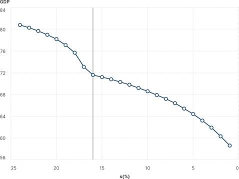
Source: Own elaboration.
Figure 3 GDP path along a capital ownership concentration process with minimum wage and unemployment insurance
Notice that GDP deceleration is diminished after the wage rate is fixed at its minimum (wmin = 0.6), but it is not at all detained; GDP keeps falling with the capital ownership concentration process. The society is more unequal and creates less wealth. Hence, an unemployment insurance program under the assumption of a minimum wage policy may be fairer than a free market adjustment, in which case the unemployed are left with no purchasing power. Although an unemployment insurance program is fairer, it is not efficient rom the viewpoint of economic activity since GDP keeps falling. Hence, as an alternative, the next section explores the impact of a universal basic income program.
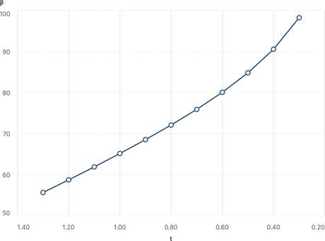
Before going into that analysis, it is worth asking ourselves whether some level of minimum wage exists that leads to better economic performance. At the beginning, it was assumed that minimum wage is politically determined at a certain level above the subsistence income. It is possible to find, however, a minimum wage rate that minimizes the unemployment rate. Figure 4 shows the result for the case in which the capital ownership concentration level is given by s = 0.10 (capitalists are 10% of the population). All other parameters are just equal to those that were assumed in the construction of Table 1.
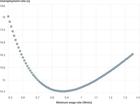
Source: Own elaboration.
Figure 4 The unemployment rate (u) versus the minimum wage rate (wmin). Notes: Parameters: s = 0.10; α = 2; β = 1.3; γ = 0.5; ϕ = 2; θ = 0.75; K = 30; N = 60.
The search grid shows that a minimum wage rate around 0.87, higher than the subsistence income (γ = 0.5), yields the lowest unemployment rate (around 14.5%). The effect of the purchasing power of the minimum wage should be balanced with the cost effect of minimum wage. Therefore, the purchasing power as a determinant of economic activity level seems to be a powerful argument in favour of setting the minimum wage rate above the subsistence income. Moreover, an optimal minimum wage rate does exist.
A Universal Basic Income Program
This section considers the economic effects of a basic income for everyone. In this situation, the economic system is modified as follows:
In this new set up, the universal basic income per person is given by b. Hence, Equations (4) and (*) in Equation System 1 become Equations (17) and In this new set up, the universal basic income per person is given by b. Hence, Equations (4) and (*) in Equation System 1 become Equations (17) and (•), the typical worker’s demand equations for manufacturing goods and food. Notice that the typical worker’s net income increases from w to w + b. As in the previous analysis, capitalists pay taxes on their returns. Hence, the typical capitalist’s returns after taxes are given by r(1─t)ke, and he/she also receives the basic income (b). Therefore, Equations (5) and (**) become Equations (18) and (••), which are the typical capitalist demand equations for manufacturing goods and food. Now, it is assumed that the government finances the universal basic income. The long-run fiscal equilibrium imposes that tax collection on capital returns equals government spending (rKet = bN ). The substitution of Equation (6) in the previous condition yields Equation (19). The solution of this economic system reveals that it might be possible to find a universal basic income per person that solves the effective demand shortage, the typical worker’s demand equations for manufacturing goods and food. Notice that the typical worker’s net income increases from w to w + b. As in the previous analysis, capitalists pay taxes on their returns. Hence, the typical capitalist’s returns after taxes are given by r(1 t)ke, and he/she also receives the basic income (b). Therefore, Equations (5) and (**) become Equations (18) and, which are the typical capitalist demand equations for manufacturing goods and food. Now, it is assumed that the government finances the universal basic income. The long-run fiscal equilibrium imposes that tax collection on capital returns equals government spending (rKet = bN ). The substitution of Equation(6) in the previous condition yields Equation (19). The solution of this economic system reveals that it might be possible to find a universal basic income per person that solves the effective demand shortage and preserves the markets equilibria. Exceptions to this rule include extreme situations of automation that will be analysed later.
The mathematical solution of this economic system with universal basic income is confined to Appendix 2.
As in the previous analysis, there are two moments of the process of capital ownership concentration: 1) an intermediate degree of capital ownership concentration (0.24 s 0.17) and 2) a high degree of capital ownership concentration (s < 0.17). In the first moment, there exists a set of prices that equilibrate the economy. Capital and labour are fully employed without government intervention. Hence, there is no need for any redistributive fiscal policy. In the second moment, capital is fully employed, but labour unemployment would arise without an income redistribution process. The high degree of capital ownership concentration forces the wage reduction until it hits its minimum level, which is set above the subsistence income.
Now, let us analyse the evolution of the variables along the capital ownership concentration process.
This process is represented with a decreasing population fraction of capitalists (see Column 1). The wage rate lowers, and the user cost of capital increases (Columns 2 and 3). This process continues until the labour remuneration is set at its minimum level. As in the previous analysis, the minimum wage rate is assumed to be equal to 0.6, a bit higher than the minimum food consumption per person. Without government intervention, the wage rate would keep falling and a social problem of unemployment would arise. Appendix 2 shows that, in this context, a tax rate on capital returns may be found so that the government finances the universal basic income program, and the economy preserves the general equilibrium through a recovery of the population’s purchasing power. The optimal tax rate, t, is null in the first moment of low capital ownership concentration and increases in the second moment with the falling s variable (see Column 4). By the same token, the optimal basic income per capita, b, is null in the first moment and increases in the second (see Column 12). Thus, under a high level of wealth concentration income, redistribution becomes more important in order to sustain the population’s purchasing power. Columns 5, 6, 7, and 8 show the equilibrium prices and varieties of both high-demand manufacturing goods and low-demand manufacturing goods. Although the typical worker’s consumption of manufacturing goods is always less diversified than the typical capitalist’s consumption of manufacturing goods (m < M), the first one increases, and the second decreases with the process of capital ownership concentration.
Hence, social inequality decreases with an optimal tax rate. The demand for capital per capitalist and the supply of capital per capitalist are equalised (ke = k) at any level of s (see Columns 9 and 10), indicating that the capital market clears. Also, the unemployment rate is always null both under the case of low capital ownership concentration with no government intervention and under the case of high capital ownership concentration with a minimum wage policy and an optimal universal basic income (see Column 17).
Food consumption of individual workers and capitalists (fw and fk, respectively) are are also defined in Table 2 as well as the demands for capital and labour from the food sector (see Columns 13 and 14), and the demands for capital and labour from the food sector are also defined (see Column 15). GDP falls with the concentration of capital ownership with no government intervention due to the shortage of the population purchasing power; but when the minimum wage is established and the universal basic income program is enacted (for s ─ 0.16), GDP increases even though the capital ownership concentration process continues in the economy (see Column 16 and Figure 5).
Table 2 The model with minimum wage and universal basic income
| s (1) | w (2) | r (3) | t (4) | p (5) | P (6) | m 7) | M (8) | k e (9) | k (10) | r(1- t)k e /w (11) | b (12) | f w (13) | f k (14) | K F = L F (15) | GDP (16) | u (17) |
|---|---|---|---|---|---|---|---|---|---|---|---|---|---|---|---|---|
| 0.24 | 1.33 | 0.67 | 0 | 1.76 | 1.83 | 020 | 0.21 | 2.08 | 2.08 | 1.04 | 0 | 0.98 | 1.02 | 29.6 | 80.8 | 0 |
| 0.23 | 1.25 | 0.75 | 0 | 1.65 | 1.74 | 0.20 | 0.28 | 2.17 | 2.17 | 1.29 | 0 | 0.93 | 1.15 | 29.4 | 80.3 | 0 |
| 0.22 | 1.17 | 0.83 | 0 | 1.55 | 1.65 | 0.19 | 0.36 | 2.27 | 2.27 | 1.60 | 0 | 0.89 | 1.30 | 29.3 | 79.7 | 0 |
| 0.21 | 1.09 | 0.91 | 0 | 1.45 | 1.57 | 0.18 | 0.46 | 2.38 | 2.38 | 1.97 | 0 | 0.84 | 1.46 | 29.1 | 79.0 | 0 |
| 0.20 | 1.01 | 0.99 | 0 | 1.35 | 1.48 | 0.16 | 0.58 | 2.50 | 2.50 | 2.45 | 0 | 0.79 | 1.64 | 28.8 | 78.2 | 0 |
| 0.19 | 0.92 | 1.08 | 0 | 1.23 | 1.39 | 0.15 | 0.73 | 2.63 | 2.63 | 3.08 | 0 | 0.74 | 1.85 | 28.5 | 77.1 | 0 |
| 0.18 | 0.82 | 1.18 | 0 | 1.10 | 1.28 | 0.12 | 0.94 | 2.78 | 2.78 | 4.02 | 0 | 0.68 | 2.11 | 28.1 | 75.7 | 0 |
| 0.17 | 0.66 | 1.34 | 0 | 0.91 | 1.12 | 0.08 | 1.32 | 2.94 | 2.94 | 5.94 | 0 | 0.59 | 2.47 | 27.4 | 73.1 | 0 |
| 0.16 | 0.6 | 1.4 | 0.068 | 0.83 | 1.07 | 0.08 | 1.44 | 3.12 | 3.13 | 6.70 | 0.06 | 0.59 | 2.56 | 27.1 | 72.2 | 0 |
| 0.15 | 0.6 | 1.4 | 0.149 | 0.83 | 1.09 | 0.12 | 1.37 | 3.33 | 3.33 | 6.41 | 0.12 | 0.63 | 2.50 | 27.2 | 72.6 | 0 |
| 0.14 | 0.6 | 1.4 | 0.227 | 0.83 | 1.11 | 0.15 | 1.31 | 3.57 | 3.57 | 6.14 | 0.18 | 0.66 | 2.45 | 27.4 | 73.0 | 0 |
| 0.13 | 0.6 | 1.4 | 0.301 | 0.83 | 1.14 | 0.18 | 1.25 | 3.85 | 3.85 | 5.87 | 0.24 | 0.70 | 2.40 | 27.5 | 73.3 | 0 |
| 0.12 | 0.6 | 1.4 | 0.371 | 0.83 | 1.17 | 0.20 | 1.19 | 4.17 | 4.17 | 5.62 | 0.30 | 0.73 | 2.35 | 27.6 | 73.7 | 0 |
| 0.11 | 0.6 | 1.4 | 0.438 | 0.83 | 1.20 | 0.23 | 1.13 | 4.55 | 4.55 | 5.39 | 0.34 | 0.75 | 2.31 | 27.7 | 74.0 | 0 |
| 0.10 | 0.6 | 1.4 | 0.501 | 0.83 | 1.25 | 0.25 | 1.07 | 5.00 | 5.00 | 5.17 | 0.39 | 0.78 | 2.27 | 27.9 | 74.4 | 0 |
| 0.09 | 0.6 | 1.4 | 0.561 | 0.83 | 1.30 | 0.28 | 1.01 | 5.56 | 5.56 | 4.98 | 0.43 | 0.80 | 2.24 | 28.0 | 74.8 | 0 |
| 0.08 | 0.6 | 1.4 | 0.617 | 0.83 | 1.36 | 0.30 | 0.95 | 6.25 | 6.25 | 4.80 | 0.47 | 0.83 | 2.22 | 28.1 | 75.1 | 0 |
| 0.07 | 0.6 | 1.4 | 0.670 | 0.83 | 1.45 | 0.31 | 0.89 | 7.14 | 7.14 | 4.65 | 0.50 | 0.85 | 2.21 | 28.2 | 75.5 | 0 |
| 0.06 | 0.6 | 1.4 | 0.720 | 0.83 | 1.56 | 0.33 | 0.83 | 8.33 | 8.33 | 4.55 | 0.54 | 0.86 | 2.22 | 28.3 | 75.8 | 0 |
| 0.05 | 0.6 | 1.4 | 0.767 | 0.83 | 1.71 | 0.34 | 0.77 | 10.00 | 10.00 | 4.51 | 0.56 | 0.88 | 2.26 | 28.5 | 76.2 | 0 |
| 0.04 | 0.6 | 1.4 | 0.810 | 0.83 | 1.95 | 0.36 | 0.71 | 12.50 | 12.50 | 4.56 | 0.59 | 0.89 | 2.35 | 28.6 | 76.6 | 0 |
| 0.03 | 0.6 | 1.4 | 0.850 | 0.83 | 2.34 | 0.37 | 0.65 | 16.67 | 16.67 | 4.82 | 0.61 | 0.91 | 2.54 | 28.7 | 76.9 | 0 |
| 0.02 | 0.6 | 1.4 | 0.887 | 0.83 | 3.11 | 0.38 | 0.60 | 25.00 | 25.00 | 5.55 | 0.63 | 0.92 | 2.98 | 28.8 | 77.3 | 0 |
| 0.01 | 0.6 | 1.4 | 0.920 | 0.83 | 5.45 | 0.39 | 0.54 | 50.00 | 50.00 | 8.19 | 0.65 | 0.93 | 4.42 | 28.9 | 77.6 | 0 |
| 0.001 | 0.6 | 1.4 | 0.948 | 0.83 | 47.45 | 0.40 | 0.49 | 500.0 | 500.0 | 59.28 | 0.66 | 0.94 | 31.48 | 29.0 | 78.0 | 0 |
Notes: Parameters: α = 2; β = 1.3; γ = 0.5; ϕ = 2; θ = 0.75; K = 30; N = 60; wmin = 0.6.
Source: own elaboration.
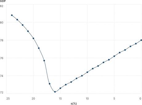
Source: own elaboration.
Figure 5 GDP path along a capital ownership concentration process with minimum wage rate and optimal universal basic income. Notes: Parameters: α = 2; β = 1.3; γ = 0.5; ϕ = 2; θ = 0.75; K = 30; N = 60; wmin = 0.6.
The economic system with an optimal universal basic income and a minimum wage is fairer than the free-market outcome. No one is unemployed, and the purchasing access to manufacturing goods is more homogeneous across the social classes when the degree of capital ownership increases. In addition, this economic policy is efficient because it recovers the society’s purchasing power, and thus GDP increases with the process of capital ownership concentration. Of course, this outcome is not free since it implies an increasing tax rate and an increasing basic income payment per person.
Figure 6 exhibits the comparative static analysis of an automation process in the manufacturing sector. It is represented by a falling requirement of marginal labour (the β coefficient falls). The population fraction of capitalists is just 10% (s = 0.10). Given the relative substitution of labour for capital in the productive manufacturing activity, a growing optimal tax rate is required in order to preserve the market equilibrium. This policy result is viable as long as the tax rate does not hit 100%; but, as Figure 6 shows, for high levels of manufacturing automation (low β), the basic income program becomes untenable. Hence, sooner or later the ongoing process of automation will imply some forms of capital property redistribution since income redistribution policies will be unable to sustain the required level of purchasing power for economic activity.
Conclusions
It would be naive to aspire that a simple economic model like the one constructed here might be a realistic representation of the complex world economy. As a matter of fact, the model construction was guided by the minimization of mathematics complexities. Notwithstanding, the increasing returns characteristic of manufacturing activities at the supply side along with the consideration of non-homothetic and satiable preferences at the demand side allow the assessment of redistributive economic policies under conditions of high capital property concentration.
The new model replicates the results of the original model (Ortiz & Castillo, 2020). First, a minimum volume of population is required in order to have a manufacturing industrial sector. Secondly, the model solutions reveal that a minimum degree of capital ownership concentration is required for the manufacturing activity to take off. Third, for intermediate degrees of capital ownership concentration, a general equilibrium solution may be found with full economic factors employment and no government intervention. Lastly, when the economic system reaches or surpasses some threshold level of capital ownership concentration, the effective demand for capital exceeds actual supply, and the opposite happens in the labour market-labour unemployment appears, and the wage ought to be fixed to a minimum level.
Thus, under the condition of high capital property concentration, two redistributive policies are considered in this paper: 1) an unemployment insurance which pays the subsistence income per unemployed person; 2) a universal basic income per capita. Both economic policies require an active government and are financed through taxation on capital returns under the assumption that all workers are paid the minimum wage rate.
The unemployment insurance program alleviates the economic situation of the unemployed, but it is not enough to counterbalance the fall in the population’s purchasing power due to the fact that the concentration of capital ownership (and income) is in very few hands. Hence, GDP falls along the process of capital ownership concentration, and income distribution worsens. As a special result, it is worth mentioning that an optimal minimum wage rate can be found. This minimum wage rate minimises the unemployment rate, and it might be above the subsistence income. Hence, the fact that the minimum wage rate is usually set above the subsistence income could be explained both for political and moral reasons as well as for economic efficiency. The economic analysis of this section is quite particular because the workings of the economy are modified when the unemployed cease to demand manufactures (the mathematical solution is given in Appendix 1).
The second redistributive policy is the payment of a universal basic income per capita. This payment could be optimally chosen such that a general economic equilibrium is preserved even under a high degree of capital ownership concentration. Two conflicting processes interact there. The process of capital ownership concentration induces a falling GDP because of the contraction of the population’s purchasing power; however, a universal basic income might overcome such an effect. The model results show that the optimal tax rate and the optimal universal basic income increase with the concentration of capital ownership. Therefore, an optimal universal basic income policy yields a growing GDP throughout the process of capital ownership concentration. The mathematical solution of the model with an optimal universal basic income is given in Appendix 2. It is worth noting, finally, that a universal basic income policy is not always viable if the degree of concentration is very high and an automation process in the manufacturing sector induces a high substitution of labour for capital. Thus, this economic model predicts that the capitalist economy requires an increasing government intervention in the redistributive sphere in order to preserve its social and economic stability.
A warning is in order. This paper explores the demand effects on economic activity from a growing degree of capital ownership concentration, but all of this is done in a static setting that ignores the productive dynamic gains from economic diversification. Hence, it would be erroneous to assume that only redistributive measures are enough. Industrial policies are also necessary to have a dynamic and virtuous economy as, according to Murphy et al., “virtually every country that experienced rapid growth of productivity and living standards over the last 200 years has done so by industrialising” (1989a, p. 1003). As Adam Smith (1776/1981) wisely proposed, “division of labour” (productive diversification) and “market size” (purchasing power) are key interactive determinants of economic development. Every government that aims at improving social welfare must promote industrialization and the population’s purchasing power.